State-space representation gives you a way to model dynamic systems using a set of first-order differential equations instead of a single higher-order transfer function. This approach is especially valuable for multi-input, multi-output (MIMO) systems and opens the door to modern control techniques like optimal control and state estimation.
Where transfer functions only show you the input-output relationship, state-space models reveal what's happening inside the system. The matrices, equations, and properties covered here form the foundation for designing controllers and observers in later units.
State-space models
State-space models describe system dynamics using a set of first-order differential equations (continuous-time) or difference equations (discrete-time), all written in matrix form. This gives you a compact, systematic way to represent even complex MIMO systems.
Difference between state-space and transfer function models
| Feature | State-Space | Transfer Function |
|---|---|---|
| System description | Internal state variables | Input-output relationship |
| MIMO handling | Direct, natural | Requires a matrix of transfer functions |
| Information provided | Internal dynamics + external behavior | External behavior only |
| Basis | Time domain (set of first-order ODEs) | Frequency domain (polynomials in ) |
Transfer functions are great for SISO analysis, but state-space models give you a fuller picture. You can always convert between the two for linear time-invariant (LTI) systems.
Advantages of state-space representation
- Handles MIMO systems in a single, unified framework
- Exposes internal structure, not just input-output behavior
- Enables state feedback controller and observer design
- Lets you check system properties like controllability and observability directly
- Supports modern control methods: optimal control (LQR), robust control, Kalman filtering
State variables
State variables are the smallest set of variables that fully describe a system's condition at any moment. They carry the system's "memory," capturing how past inputs have shaped the current state.
Definition of state variables
If you know the state variables at some time and the input for all , you can determine the future behavior of the system completely. That's what makes them the minimum set needed to characterize the system.
Selection of state variables
The choice of state variables isn't unique. For a mechanical system, you might pick position and velocity. For an electrical circuit, capacitor voltages and inductor currents are natural choices. You could also use more abstract mathematical quantities like error signals or their integrals.
What matters is that your selection:
- Uses the minimum number of variables (equal to the system order)
- Leads to a representation that is controllable and observable (when possible)
State-space equations
The state-space description consists of two equations: the state equation (how internal states evolve) and the output equation (what you can measure).
General form of state-space equations
State equation (describes the dynamics):
- : state vector ()
- : input vector ()
- : state matrix ()
- : input matrix ()
Output equation (relates states to measurements):
- : output vector ()
- : output matrix ()
- : feedthrough matrix ()
Together, these four matrices completely define the LTI system.
State equation vs output equation
The state equation governs how the internal states change over time. It captures the system's dynamics. The output equation is purely algebraic: it tells you what combination of states and inputs produces the measured output at each instant. Think of the state equation as the "engine" and the output equation as the "dashboard."
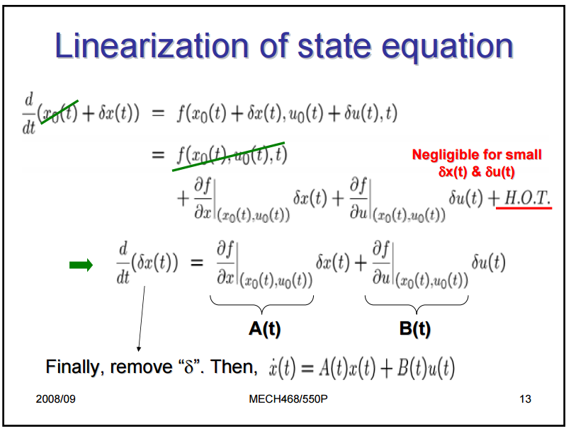
Linearization of nonlinear systems
Most real systems are nonlinear, but state-space tools are built for linear systems. To bridge this gap, you linearize around an operating point (also called an equilibrium point):
- Define the nonlinear system: ,
- Find an equilibrium point where
- Compute the Jacobian matrices (partial derivatives) of and evaluated at
- The resulting matrices become your for the linearized model
The linearized model is only accurate near the operating point. If the system moves far from that point, the approximation breaks down.
State-space matrices
State matrix A
The matrix () describes how the states interact with each other in the absence of any input. Its eigenvalues directly determine system stability and natural response:
- All eigenvalues with negative real parts → system is stable
- Any eigenvalue with a positive real part → system is unstable
- Eigenvalues with zero real parts → marginally stable (needs further analysis)
Input matrix B
The matrix () maps external inputs to the state derivatives. Each column of shows how one particular input influences all the state variables. If a column is all zeros, that input has no direct effect on the states.
Output matrix C
The matrix () determines which state variables (or combinations of them) appear in the output. Each row of corresponds to one output measurement.
Feedthrough matrix D
The matrix () represents any direct path from input to output that bypasses the state dynamics entirely. In many physical systems, because inputs must propagate through the system's dynamics before affecting the output. A nonzero means the output responds instantaneously to input changes.
Controllability
Controllability tells you whether you can drive the system from any initial state to any desired state in finite time using the available inputs. If a system isn't fully controllable, there are internal modes you simply cannot influence, no matter what input you apply.
Definition of controllability
A system is controllable if, for any initial state and any desired final state , there exists an input that transfers the system from to in finite time.
Controllability matrix
For an LTI system with states, the controllability matrix is:
This matrix has dimensions (for inputs).
Controllability tests
- Rank test: The system is controllable if and only if (full row rank).
- PBH test: The system is controllable if and only if for every eigenvalue of . This test is particularly useful for identifying which modes are uncontrollable.
Controllable canonical form
The controllable canonical form is a specific arrangement of the state-space matrices where the controllability structure is immediately visible. In this form, takes a companion matrix structure and has a single nonzero entry. This form is especially useful for designing state feedback controllers via pole placement, since the feedback gains map directly to the desired characteristic polynomial coefficients.
Observability
Observability is the dual of controllability. Instead of asking "can you control every state?", it asks "can you determine every state from the outputs?"
Definition of observability
A system is observable if the initial state can be uniquely determined from knowledge of the input and output over a finite time interval.
Observability matrix
For an LTI system with states, the observability matrix is:
This matrix has dimensions (for outputs).
Observability tests
- Rank test: The system is observable if and only if (full column rank).
- PBH test: The system is observable if and only if for every eigenvalue of .
Observable canonical form
The observable canonical form is the dual of the controllable canonical form. Here, and are structured so that the observability properties are explicit. This form is the natural starting point for designing state observers.
Duality between controllability and observability: A system is controllable if and only if the dual system is observable. This means any result you prove for controllability has a corresponding observability result, and vice versa.
Transformations of state-space models
Different choices of state variables lead to different matrices, but the underlying system is the same. Transformations let you switch between representations while preserving the input-output behavior.
Similarity transformations
Given a nonsingular matrix , define a new state vector . The transformed matrices are:
Key properties preserved under similarity transformations:
- Eigenvalues of (and therefore stability)
- Transfer function
- Controllability and observability
Coordinate transformations
Coordinate transformations are similarity transformations chosen to simplify the representation. You might rotate, scale, or translate the state variables to decouple the dynamics or align states with physically meaningful quantities. For example, diagonalizing (when possible) decouples the state equations so each state evolves independently.
Canonical forms
Canonical forms are standardized representations with specific structural properties:
- Controllable canonical form: highlights controllability, useful for pole placement
- Observable canonical form: highlights observability, useful for observer design
- Jordan canonical form: diagonalizes (or puts it in Jordan blocks for repeated eigenvalues), revealing the system's natural modes directly
Solution of state-space equations
State transition matrix
The state transition matrix maps the state at time to the state at time for the unforced (zero-input) system. It satisfies:
The complete solution (with input) is:
The first term is the zero-input response (due to initial conditions), and the integral is the zero-state response (due to the input).

Matrix exponential
For LTI systems, the state transition matrix equals the matrix exponential:
The matrix exponential is defined by the power series:
Computing directly from the series is rarely practical. Common methods include:
- Diagonalization: if , then
- Laplace transform:
- Cayley-Hamilton theorem
Laplace transform approach
Taking the Laplace transform of :
-
Transform:
-
Rearrange:
-
Solve:
-
Inverse Laplace transform to get
This approach converts differential equations into algebraic equations, which is often easier to handle.
Numerical methods for simulation
When analytical solutions are impractical (large systems, time-varying parameters, nonlinearities), numerical methods approximate the solution by stepping through time:
- Euler method: simplest, but can be inaccurate for stiff systems
- Runge-Kutta methods (e.g., RK4): good balance of accuracy and computational cost
- Dormand-Prince: adaptive step-size variant of Runge-Kutta, used by MATLAB's
ode45
These methods discretize the continuous equations and compute from iteratively.
Steady-state response
Once transients decay, the system settles into its steady-state behavior. Understanding this long-term behavior is critical for evaluating system performance.
Equilibrium points
An equilibrium point is a state where the system stays put if undisturbed. You find it by setting :
For a given constant input , the equilibrium state is (assuming is invertible). If is singular, equilibrium points may not exist or may not be unique.
Stability of equilibrium points
Stability determines whether the system returns to equilibrium after a small perturbation:
- Asymptotically stable: all eigenvalues of have strictly negative real parts. The system returns to equilibrium.
- Marginally stable: eigenvalues on the imaginary axis (with no repeated eigenvalues there), none with positive real parts. The system neither grows nor decays.
- Unstable: at least one eigenvalue has a positive real part. Perturbations grow over time.
For nonlinear systems, Lyapunov stability theory provides tools beyond eigenvalue analysis.
Steady-state error
Steady-state error is the persistent difference between the desired output and the actual output after transients have died out. You can analyze it using:
- The final value theorem: , where is the error in the Laplace domain
- The steady-state gain of the system, which depends on the DC gain
The system type (number of integrators) determines how well it tracks step, ramp, and parabolic inputs.
Relationship between state-space and transfer function models
Obtaining transfer functions from state-space models
Starting from the state-space equations, take the Laplace transform and eliminate the state vector to get:
This is the transfer function matrix. For a SISO system, is a single rational function of . For MIMO systems, it's a matrix where each entry relates the -th input to the -th output.
Minimal realization of transfer functions
A given transfer function can be realized by infinitely many state-space models. A minimal realization uses the fewest possible state variables and is both controllable and observable. If your realization has uncontrollable or unobservable modes, those correspond to pole-zero cancellations in the transfer function that hide internal dynamics.
Techniques for finding minimal realizations include Gilbert's method and Kalman decomposition, which separates the state space into controllable/observable, controllable/unobservable, uncontrollable/observable, and uncontrollable/unobservable parts.
Applications of state-space representation
Control system design
State feedback controllers use the form , where is a gain matrix chosen to place the closed-loop eigenvalues of at desired locations. This is pole placement. For optimal performance, the LQR (Linear Quadratic Regulator) computes by minimizing a cost function that balances state deviations against control effort.
Observer design
When you can't measure all state variables directly, an observer estimates them. The Luenberger observer uses the model plus output error correction:
The observer gain is chosen so that the estimation error decays quickly. The eigenvalues of determine how fast the observer converges. Observability is required for this design to work.
Kalman filtering
The Kalman filter is the optimal observer for systems with Gaussian process and measurement noise. It recursively updates the state estimate by combining the model prediction with noisy measurements, minimizing the mean square estimation error. Applications include GPS navigation, robot localization, and sensor fusion.
Optimal control
Optimal control finds the input that minimizes a cost function, typically of the form:
where penalizes state deviations and penalizes control effort. The solution for LTI systems is the LQR, which yields a constant state feedback gain. Combining LQR with a Kalman filter gives LQG (Linear Quadratic Gaussian) control, a powerful framework for handling both performance optimization and noise.