14.3 Applications of the central limit theorem

Approximating Probabilities with CLT

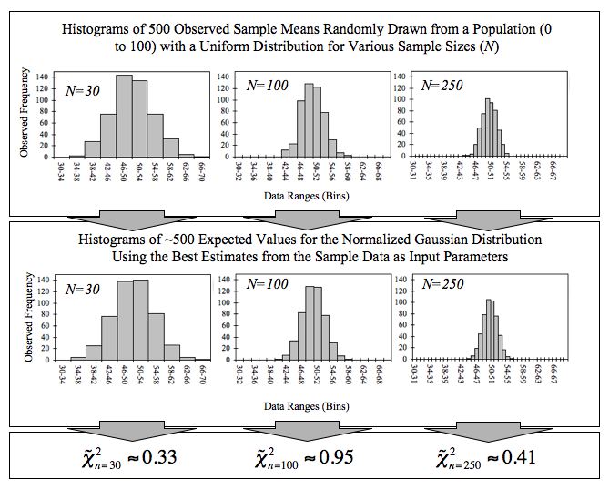
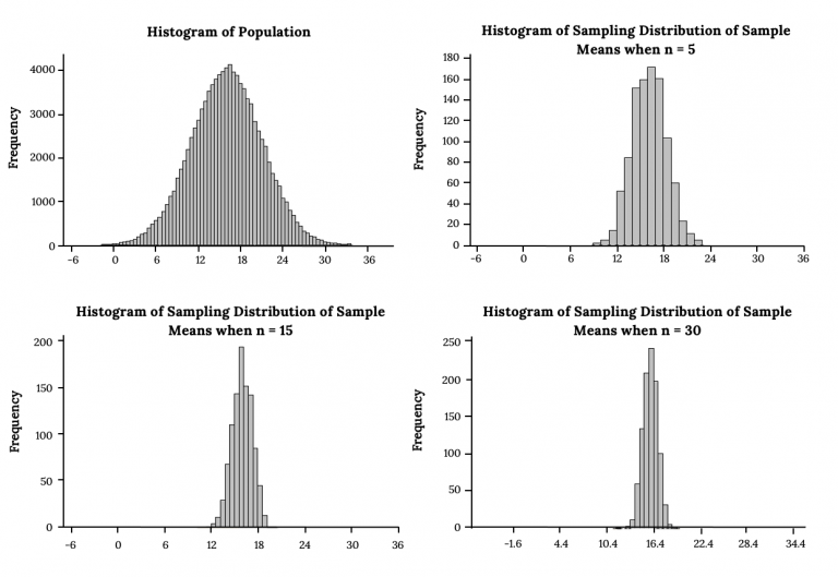
The Central Limit Theorem (CLT) says that when you take the mean of a large enough sample, that mean will follow an approximately normal distribution, regardless of what the original population looks like. This is powerful because it lets you use normal distribution tools (z-tables, standard normal calculations) on data that isn't normal at all.

Fundamentals of CLT

As sample size increases, the sampling distribution of the sample mean approaches a normal distribution with:

• Mean equal to the population mean $\mu$
• Standard error equal to $\frac{\sigma}{\sqrt{n}}$

The conventional guideline is that $n \geq 30$ is "large enough" for the CLT to kick in, though populations that are already close to normal need smaller samples, and heavily skewed populations may need larger ones.

To find probabilities involving sample means, you convert to a z-score:

$z = \frac{\bar{x} - \mu}{\sigma / \sqrt{n}}$

where $\bar{x}$ is the sample mean, $\mu$ is the population mean, $\sigma$ is the population standard deviation, and $n$ is the sample size.

This works even when the underlying population is uniform, exponential, or some other non-normal shape.

Probability Calculations

Once you have a z-score, you look up the corresponding probability using a standard normal table (or calculator).

Typical problem types:

• What's the probability that the sample mean falls within a specific range? Convert both endpoints to z-scores and find the area between them.
• What's the probability that the sample mean exceeds a certain value? Convert to a z-score and find the area in the upper tail.

Example: Suppose a population has $\mu = 50$ and $\sigma = 10$. You draw a sample of $n = 64$. What's the probability that $\bar{x} > 52$?

1. Compute the standard error: $\frac{10}{\sqrt{64}} = 1.25$

2. Compute the z-score: $\frac{52 - 50}{1.25} = 1.6$

3. Look up $P(Z > 1.6) \approx 0.0548$

So there's about a 5.5% chance the sample mean exceeds 52.

Confidence Intervals with CLT

A confidence interval gives you a range of plausible values for the population mean based on your sample data.

Constructing Confidence Intervals

The general formula is:

$\bar{x} \pm (\text{critical value}) \times \frac{\sigma}{\sqrt{n}}$

Here's how to build one step by step:

1. Compute the sample mean $\bar{x}$.
2. Determine the standard error $\frac{\sigma}{\sqrt{n}}$ (or $\frac{s}{\sqrt{n}}$ if $\sigma$ is unknown).
3. Choose your confidence level (common choices: 90%, 95%, 99%).
4. Find the critical value. For large samples using the z-distribution, the critical values are approximately 1.645 (90%), 1.96 (95%), and 2.576 (99%).
5. Calculate the margin of error: critical value $\times$ standard error.
6. Form the interval: $\bar{x} - \text{margin of error}$ to $\bar{x} + \text{margin of error}$.

Three factors control how wide the interval is:

• Sample size: Larger $n$ shrinks the standard error, giving a narrower interval.
• Population variability: Higher $\sigma$ means a wider interval.
• Confidence level: Higher confidence (say 99% vs. 95%) requires a wider interval.

Interpretation and Application

A 95% confidence interval does not mean there's a 95% chance the population mean is inside your particular interval. It means that if you repeated the sampling process many times, about 95% of the resulting intervals would contain the true mean.

The CLT is what makes these intervals approximately valid for large samples, even when the population isn't normal. Without the CLT, you'd need to know (or assume) the population's exact distribution to build a confidence interval.

Hypothesis Testing with CLT

Hypothesis testing uses sample data to evaluate a claim about a population parameter. The CLT makes this possible for means even when the population distribution is unknown.

Fundamentals of Hypothesis Testing

The setup involves two competing statements:

• Null hypothesis ($H_0$): The default claim, typically "no effect" or "no difference." For example, $H_0: \mu = \mu_0$.
• Alternative hypothesis ($H_1$): What you're trying to find evidence for. This can be one-sided ($\mu > \mu_0$ or $\mu < \mu_0$) or two-sided ($\mu \neq \mu_0$).

The test statistic measures how far your sample result is from what $H_0$ predicts:

$z = \frac{\bar{x} - \mu_0}{\sigma / \sqrt{n}}$

where $\mu_0$ is the hypothesized population mean. Thanks to the CLT, this statistic is approximately standard normal for large $n$, so you can use z-tables to assess the result.

Testing Approaches and Considerations

There are two common ways to make a decision:

P-value approach:

1. Calculate the test statistic $z$.
2. Find the p-value: the probability of observing a result at least as extreme as yours, assuming $H_0$ is true.
3. If the p-value $\leq \alpha$ (your significance level, often 0.05), reject $H_0$.

Critical value approach:

1. Calculate the test statistic $z$.
2. Determine the critical value(s) from the significance level and test type (one-tailed or two-tailed).
3. If $z$ falls in the rejection region, reject $H_0$.

Both approaches give the same conclusion. The p-value approach is more common because it tells you how much evidence you have against $H_0$, not just whether you crossed a threshold.

Two types of errors to watch for:

• Type I error: Rejecting $H_0$ when it's actually true. The probability of this equals $\alpha$.
• Type II error: Failing to reject $H_0$ when it's actually false. Harder to control, and depends on the true parameter value and sample size.

Limitations of CLT

Assumptions and Sample Size Considerations

The CLT requires that the random variables be independent and identically distributed (i.i.d.). This assumption breaks down with time series data (where observations are correlated) or clustered data (where observations within groups are more similar).

Sample size matters more than the $n \geq 30$ rule suggests:

• For symmetric or mildly skewed populations, $n = 30$ usually works fine.
• For heavily skewed distributions (exponential, Pareto), you may need $n$ in the hundreds before the sampling distribution looks normal.
• For distributions with very heavy tails, like the Cauchy distribution, the CLT doesn't apply at all because the population mean and variance don't exist.

One common misconception: the CLT does not say that your data becomes normal as you collect more of it. It says the distribution of the sample mean (across many hypothetical samples) becomes normal.

Scope and Alternative Methods

The CLT applies to sums and means of random variables. It does not automatically extend to other statistics like medians, ranges, or variances.

For other types of data, different tools are more appropriate:

• Proportions: The CLT can approximate binomial proportions when $np$ and $n(1-p)$ are both at least 5 or 10 (depending on the convention). Outside that range, use the binomial distribution directly.
• Counts of rare events: The Poisson distribution is typically a better model than a normal approximation.
• Small samples from skewed populations: Consider exact methods, bootstrapping, or non-parametric tests rather than relying on the CLT.