Cumulative distribution functions (CDFs) are essential tools in probability theory. They give us a complete picture of a random variable's behavior, showing the likelihood of it falling below any given value. CDFs are versatile, applicable to both discrete and continuous variables.
CDFs connect to the broader study of continuous random variables by providing a unified framework for analysis. They allow us to calculate probabilities, find percentiles, and generate random samples. Understanding CDFs is crucial for grasping more advanced concepts in probability and statistics.
Cumulative Distribution Functions
Definition and Basic Properties
Top images from around the web for Definition and Basic Properties
Cumulative distribution function - Wikipedia View original
Is this image relevant?
1 of 3
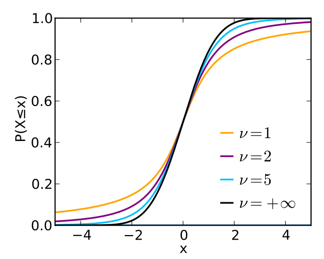
Cumulative distribution function (CDF) F(x) for random variable X represents probability X takes value less than or equal to x F(x)=P(X≤x)
Non-decreasing function F(x1)≤F(x2) for all x1<x2
Approaches 0 as x approaches negative infinity and 1 as x approaches positive infinity
Continuous function for continuous random variables
Right-continuous, meaning limx→x0+F(x)=F(x0)
Step function with jumps at possible values of X for discrete random variables
Probability of X taking specific value a given by P(X=a)=F(a)−limx→a−F(x)
Advanced Properties and Applications
Used to generate random samples from given distribution through inverse CDF method
Derives statistical measures (expected values, variances) through integration techniques
Analyzes transformations of random variables, particularly for monotonic functions
Determines stochastic dominance between different random variables or distributions
Represents failure distribution in reliability analysis, with complement (1 - F(x)) as reliability function
Utilized in hypothesis testing (Kolmogorov-Smirnov tests) to compare sample distributions to theoretical distributions
Analyzes relationships between multiple random variables using joint CDFs and marginal CDFs in multivariate settings
CDFs vs PDFs
Relationship and Conversion
Probability density function (PDF) f(x) represents derivative of CDF F(x) for continuous random variables f(x)=dxdF(x)
CDF obtained by integrating PDF F(x)=∫−∞xf(t)dt
Area under PDF curve between points a and b represents probability P(a<X≤b)=F(b)−F(a)
For discrete random variables, probability mass function (PMF) replaces PDF, CDF becomes sum of PMF values up to and including x
PDF must be non-negative and integrate to 1 over entire domain, corresponding to CDF ranging from 0 to 1
Discontinuities in CDF correspond to point masses in probability distribution, represented by delta functions in PDF for continuous random variables
Comparative Analysis
CDF provides cumulative probabilities, while PDF gives probability density at specific points
CDF always exists for all random variables, while PDF exists only for continuous random variables
CDF ranges from 0 to 1, while PDF can take any non-negative value
CDF used directly for calculating probabilities, while PDF requires integration
CDF always continuous from the right, while PDF may have discontinuities
CDF monotonically increasing, while PDF can increase or decrease
CDF used in stochastic ordering and reliability analysis, while PDF used in maximum likelihood estimation and information theory
Probabilities with CDFs
Basic Probability Calculations
Probability of X being less than or equal to specific value a given directly by CDF P(X≤a)=F(a)
Probability of X being greater than specific value a calculated as P(X>a)=1−F(a)
Probability of X falling within interval [a, b] calculated as P(a≤X≤b)=F(b)−F(a)
For continuous random variables, P(X=a)=0, so P(a<X≤b)=P(a≤X≤b)=F(b)−F(a)
Median of distribution found by solving F(x)=0.5
Percentiles of distribution calculated by finding inverse of CDF (quantile function)
For discrete random variables, probabilities of specific values found by subtracting consecutive CDF values P(X=x)=F(x)−F(x−)
Advanced Probability Applications
Calculating joint probabilities for multiple random variables using multivariate CDFs
Determining conditional probabilities using CDFs of marginal and joint distributions
Computing probabilities for functions of random variables through CDF transformations
Analyzing order statistics using CDFs (finding distribution of maximum or minimum of sample)
Calculating probabilities in reliability engineering (system failure probabilities)
Determining probabilities in financial risk management (Value at Risk calculations)
Computing probabilities in queueing theory (waiting time distributions)
Continuous Random Variables with CDFs
Analysis and Problem Solving
Generate random samples from given distribution using inverse CDF method
Derive statistical measures (expected values, variances) through integration techniques
Analyze transformations of random variables, particularly for monotonic functions
Determine stochastic dominance between different random variables or distributions
Represent failure distribution in reliability analysis, with complement (1 - F(x)) as reliability function
Utilize in hypothesis testing (Kolmogorov-Smirnov tests) to compare sample distributions to theoretical distributions
Analyze relationships between multiple random variables using joint CDFs and marginal CDFs in multivariate settings
Applications in Various Fields
Economics calculate income distributions and inequality measures (Gini coefficient)
Finance model asset returns and price options (Black-Scholes model)
Engineering analyze system reliability and component lifetimes (Weibull distribution)
Physics study particle decay times and radioactive decay (exponential distribution)
Environmental science model extreme weather events (generalized extreme value distribution)
Quality control determine process capability and tolerance limits (normal distribution)
Actuarial science assess insurance risks and set premiums (Pareto distribution)
Key Terms to Review (16)
Cumulative Distribution Function (CDF): The cumulative distribution function (CDF) is a function that describes the probability that a random variable takes on a value less than or equal to a certain value. It provides a complete description of the probability distribution of a random variable, whether it is discrete or continuous. By calculating probabilities for different values, the CDF helps in understanding how values are distributed within a dataset and is essential for various statistical analyses.
Calculating probabilities: Calculating probabilities involves determining the likelihood of a specific event occurring within a defined set of outcomes. This process is essential for understanding how random variables behave, and it provides insight into predicting future events based on observed data. In the context of cumulative distribution functions, calculating probabilities allows us to evaluate the likelihood of outcomes falling within particular ranges, which is crucial for statistical analysis.
Probability Density Function: A probability density function (PDF) describes the likelihood of a continuous random variable taking on a particular value. Unlike discrete variables, which use probabilities for specific outcomes, a PDF represents probabilities over intervals, making it essential for understanding continuous distributions and their characteristics.
Cumulative Distribution Function: The cumulative distribution function (CDF) of a random variable is a function that describes the probability that the variable will take a value less than or equal to a specific value. The CDF provides a complete description of the distribution of the random variable, allowing us to understand its behavior over time and its potential outcomes in both discrete and continuous contexts.
Inverse cdf: The inverse cumulative distribution function (inverse cdf) is a function that takes a probability value and returns the corresponding value of the random variable. This function is essential in understanding how probabilities relate to outcomes, allowing for the determination of quantiles and enabling simulations of random variables by transforming uniform random variables into ones with the desired distribution.
Step Function: A step function is a piecewise constant function that takes a constant value on each interval of its domain and jumps to a different constant value at specific points. These functions are particularly useful in probability and statistics as they can represent cumulative distribution functions, which indicate the probability that a random variable is less than or equal to a certain value. Understanding step functions helps in visualizing distributions and analyzing discrete random variables.
Standardization of Random Variables: Standardization of random variables is the process of transforming a random variable into a standard score, typically referred to as a z-score. This transformation allows for comparison between different random variables by converting them into a common scale with a mean of 0 and a standard deviation of 1. This technique is essential when analyzing the cumulative distribution functions as it helps in understanding how far a particular value is from the mean in terms of standard deviations.
Quantile Function: The quantile function is a statistical tool that provides the value below which a given percentage of observations in a dataset falls. It serves as the inverse of the cumulative distribution function (CDF), meaning it allows one to determine a specific data value corresponding to a given cumulative probability. This concept is vital in understanding the distribution of continuous random variables, as it helps in analyzing and interpreting data through various applications.
Limits of cdf: The limits of the cumulative distribution function (CDF) describe the behavior of the CDF as it approaches its extreme values. Specifically, the CDF will approach 0 as the variable approaches negative infinity and will approach 1 as the variable approaches positive infinity. This property is fundamental in understanding how probabilities accumulate over the range of a random variable.
Plotting CDF: Plotting the cumulative distribution function (CDF) involves graphing a function that describes the probability that a random variable takes on a value less than or equal to a specific point. The CDF provides a complete description of the distribution of a random variable and can be used for both discrete and continuous cases. Understanding how to plot a CDF is essential for visualizing probabilities and making informed decisions based on statistical data.
Non-decreasing function: A non-decreasing function is a type of mathematical function where, as the input values increase, the output values do not decrease. This means that for any two points in its domain, if one point is less than or equal to another, then the function's value at the first point is less than or equal to its value at the second. This characteristic is particularly important in understanding cumulative distribution functions, which summarize the probability of a random variable taking on values less than or equal to a specified value.
Law of Total Probability: The law of total probability is a fundamental principle that relates marginal probabilities to conditional probabilities, allowing for the calculation of the probability of an event based on a partition of the sample space. It connects different aspects of probability by expressing the total probability of an event as the sum of its probabilities across mutually exclusive scenarios or conditions.
Central Limit Theorem: The Central Limit Theorem (CLT) states that, regardless of the original distribution of a population, the sampling distribution of the sample mean will approach a normal distribution as the sample size increases. This is a fundamental concept in statistics because it allows for making inferences about population parameters based on sample statistics, especially when dealing with larger samples.
Normal distribution: Normal distribution is a continuous probability distribution that is symmetric around its mean, showing that data near the mean are more frequent in occurrence than data far from the mean. This bell-shaped curve is crucial in statistics because it describes how many real-valued random variables are distributed, allowing for various interpretations and applications in different areas.
Exponential distribution: The exponential distribution is a continuous probability distribution that describes the time between events in a Poisson process, where events occur continuously and independently at a constant average rate. It is particularly useful for modeling the time until an event occurs, such as the lifespan of electronic components or the time until a customer arrives at a service point.
Statistical inference: Statistical inference is the process of drawing conclusions about a population based on a sample of data. It allows researchers to make predictions or generalizations and assess the reliability of those conclusions, often using concepts like expected value, variance, and distributions to quantify uncertainty.