🎲Intro to Probability Unit 5 Review
5.1 Concept of discrete random variables
5.1 Concept of discrete random variables
Unit & Topic Study Guides
Intro to Probability: Sample Spaces
Probability Axioms and Properties
Counting: Permutations and Combinations
Conditional Probability & Independence
Discrete Random Variables & Distributions
Continuous Variables & Distributions
Expectation and Variance of Random Variables
Discrete Distributions: Bernoulli to Poisson
Continuous Distributions: Uniform to Normal
Joint Probability & Independence
Covariance and Correlation
Total Probability and Bayes' Theorem
Moment and Probability Generating Functions
Limit Theorems: LLN and Central Limit
Discrete Random Variables
Discrete random variables let you assign numbers to the outcomes of random processes, turning uncertain events into something you can analyze mathematically. They're the foundation for modeling anything you can count: coin flips, defective products on an assembly line, customers walking through a door.
This section covers what makes a random variable "discrete," how to represent one mathematically, and how discrete variables differ from continuous ones.
Discrete Random Variables
Definition and Key Properties
A discrete random variable is a variable that takes on a countable number of distinct values, each with a specific probability attached to it. "Countable" means you could list the possible values out, even if that list is infinitely long (like all positive integers).
These variables typically come from counting processes or experiments with a finite set of outcomes. A few core ideas define how they work:
- The probability mass function (PMF) assigns a probability to each possible value. It tells you exactly how likely each outcome is.
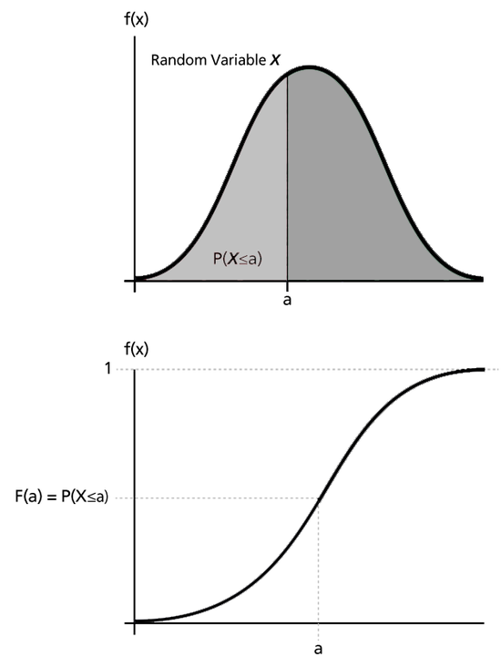
- The cumulative distribution function (CDF) tells you the probability that the variable is less than or equal to a given value. For discrete variables, the CDF is a step function since it jumps at each possible value.
- The probabilities across all possible values must sum to 1. This follows from the law of total probability: something has to happen, so the total probability is always 1.
- You can summarize a discrete random variable using its expected value (mean), variance, and standard deviation, all of which are covered below.
Mathematical Representation
The PMF is written as:
where is the random variable and is a specific value it can take. For example, if represents the result of rolling a fair die, then .
The CDF sums up probabilities for all values up to :
The expected value (or mean) is a weighted average of all possible values, weighted by their probabilities:
Variance measures how spread out the values are around the mean:
And standard deviation is just the square root of variance, which puts the spread back into the original units:
Real-World Examples of Discrete Variables
Counting Scenarios
Discrete random variables show up whenever you're counting something:
- Number of customers entering a store in a given hour (could be 0, 1, 2, 3, ...)
- Defective items in a manufacturing batch of 500 (could be 0 through 500)
- Email messages received in a day
- Car accidents at an intersection per month
- Number of children in a randomly selected family
- Goals scored in a soccer match
Notice that all of these produce whole numbers, and you could list every possible value.
Experimental Outcomes
Many probability experiments also produce discrete outcomes:
- Rolling a die gives values 1 through 6 on each roll
- Flipping a coin 10 times and counting heads gives values 0 through 10
- Drawing cards from a deck without replacement (tracking which cards appear)
- Number of successful free throws out of 20 attempts (values 0 through 20)
The key pattern: if you can count the result rather than measure it on a continuous scale, you're dealing with a discrete random variable.
Discrete vs. Continuous Variables
Key Differences
| Feature | Discrete | Continuous |
|---|---|---|
| Possible values | Countable, distinct | Any value in a range |
| Probability function | PMF (probability mass function) | PDF (probability density function) |
| Probability of exact value | Can be nonzero (e.g., ) | Always zero for any single point |
| CDF shape | Step function (jumps at each value) | Smooth, continuous curve |
| Calculations use | Summation () | Integration () |
| Typical source | Counting | Measuring |
The most important distinction to remember: for a discrete variable, you can ask "what's the probability of exactly this value?" and get a meaningful answer. For a continuous variable, you can only ask about ranges.

Examples and Applications
- Discrete: number of heads in 20 coin flips, students absent from class, items in inventory
- Continuous: height, weight, time to complete a task, temperature
Some variables can be treated either way depending on context. Age recorded in whole years is discrete, but exact age (27.4386... years) is continuous. The choice depends on how you're measuring and what model fits your situation.
Random Variables and Probability Distributions
Fundamental Concepts
A probability distribution is the complete description of a random variable: all its possible values and their associated probabilities. For discrete variables, the PMF is the distribution. Once you have it, you can derive everything else (the CDF, expected value, variance, etc.).
One important theoretical result: the law of large numbers says that as you observe more and more outcomes of a random variable, the sample mean will get closer and closer to the expected value. This is why expected value matters in practice, not just in theory.
Common Discrete Distributions
You'll encounter several named distributions throughout this course. Here's a preview of the most important ones:
- Binomial distribution: models the number of successes in a fixed number of independent trials, each with the same probability of success. Example: number of heads in 10 coin flips.
- Poisson distribution: models the number of events occurring in a fixed interval of time or space, when events happen independently at a constant average rate. Example: number of calls a help desk receives per hour.
- Geometric distribution: models the number of trials needed to get the first success. Example: how many times you roll a die before getting a 6.
- Negative binomial distribution: generalizes the geometric by modeling the number of failures before a specified number of successes.
Each of these distributions has its own PMF formula, expected value, and variance, which you'll work with in upcoming sections.
When you have multiple random variables together, a joint probability distribution describes their combined behavior, and you can extract marginal distributions from it to study each variable individually.