Variance and are key measures in probability, helping us understand how data spreads out from the average. These tools are crucial for assessing risk, quality control, and making statistical inferences across various fields.

Calculating variance involves squaring deviations from the mean, while standard deviation is the square root of variance. For both discrete and continuous variables, we'll explore formulas, examples, and important properties that make these concepts fundamental in probability theory.

Variance and Standard Deviation

Definition and Basic Properties

Top images from around the web for Definition and Basic Properties
  • Variance measures variability in a random variable quantifying how far numbers spread out from their average value
  • Denoted as or (X), defined as of squared deviation from mean: Var(X)=E[(X[μ](https://www.fiveableKeyTerm:μ))2]Var(X) = E[(X - [μ](https://www.fiveableKeyTerm:μ))²]
  • Standard deviation equals square root of variance denoted as σ(X) or expressed in same units as original data
  • Variance remains non-negative equaling zero only when random variable is constant (no variability)
  • Demonstrates non-linearity Var(aX)=a2Var(X)Var(aX) = a²Var(X) for any constant a
  • For X and Y, variance of sum equals sum of individual variances: Var(X+Y)=Var(X)+Var(Y)Var(X + Y) = Var(X) + Var(Y)
  • Standard deviation property for constant a and random variable X: SD(aX)=aSD(X)SD(aX) = |a|SD(X)

Interpretation and Significance

  • Provides measure of spread or dispersion in dataset
  • Larger variance indicates greater variability in data points (stock prices)
  • Smaller variance suggests data points cluster closely around mean (consistent product quality)
  • Used in , quality control, and
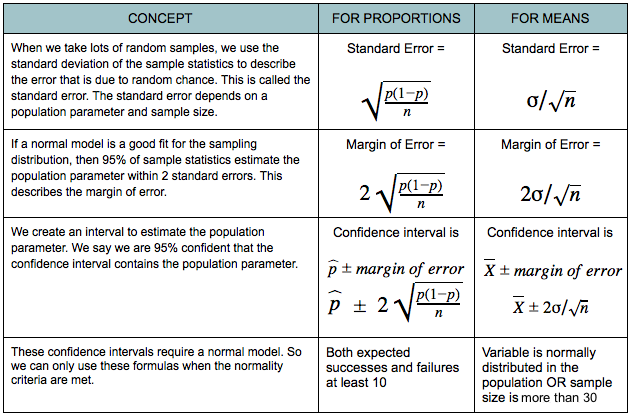
  • Plays crucial role in hypothesis testing and confidence interval construction
  • Helps in comparing datasets with different units or scales
  • Utilized in various fields (finance, engineering, social sciences) to quantify uncertainty and variability

Calculating Variance and Standard Deviation
Discrete Random Variables

  • For discrete random variable X with probability mass function p(x), variance calculated using formula: Var(X)=Σ(xμ)2p(x)Var(X) = Σ(x - μ)²p(x)
  • Expected value (mean) calculated first: μ=[E(X)](https://www.fiveableKeyTerm:e(x))=Σxp(x)μ = [E(X)](https://www.fiveableKeyTerm:e(x)) = Σxp(x)
  • Standard deviation obtained by taking square root: SD(X)=Var(X)SD(X) = √Var(X)
  • Calculation involves summing over all possible values of X in sample space
  • Alternative formula for variance: Var(X)=E(X2)[E(X)]2Var(X) = E(X²) - [E(X)]² where E(X2)=Σx2p(x)E(X²) = Σx²p(x)
  • Be aware of built-in functions for calculating variance and standard deviation in statistical software
  • Apply formulas to common discrete distributions (Binomial, Poisson, Geometric)

Calculation Examples

  • For a fair six-sided die, calculate variance:
    • p(x) = 1/6 for x = 1, 2, 3, 4, 5, 6
    • μ = E(X) = (1+2+3+4+5+6)/6 = 3.5
    • Var(X) = Σ(x - 3.5)²(1/6) = 2.917
  • For a biased coin with P(Heads) = 0.6, P(Tails) = 0.4:
    • X = 1 for Heads, X = 0 for Tails
    • μ = E(X) = 1(0.6) + 0(0.4) = 0.6
    • Var(X) = (1 - 0.6)²(0.6) + (0 - 0.6)²(0.4) = 0.24

Variance and Standard Deviation for Continuous Variables

Computation Methods

  • For continuous random variable X with probability density function f(x), variance calculated using integral: Var(X)=(xμ)2f(x)dxVar(X) = ∫(x - μ)²f(x)dx
  • Expected value (mean) calculated first: μ=E(X)=xf(x)dxμ = E(X) = ∫xf(x)dx
  • Standard deviation obtained by taking square root: SD(X)=Var(X)SD(X) = √Var(X)
  • Calculation involves integrating over entire support of probability density function
  • Alternative formula for variance: Var(X)=E(X2)[E(X)]2Var(X) = E(X²) - [E(X)]² where E(X2)=x2f(x)dxE(X²) = ∫x²f(x)dx
  • Familiarize with specific variance formulas for common continuous distributions (Normal, Exponential, Uniform)
  • Understand integration techniques or statistical software use for complex continuous distributions

Application to Specific Distributions

  • For Uniform distribution U(a,b):
    • Variance formula: Var(X)=(ba)2/12Var(X) = (b-a)²/12
    • Example: U(0,1) has variance (1-0)²/12 = 1/12 ≈ 0.0833
  • For Exponential distribution with rate parameter λ:
    • Variance formula: Var(X)=1/λ2Var(X) = 1/λ²
    • Example: Exponential(0.5) has variance 1/(0.5)² = 4
  • For Normal distribution N(μ,σ²):
    • Variance directly given as σ²
    • Example: N(0,1) (standard normal) has variance 1

Variance Properties for Independent Variables

Additive Properties

  • Variance of sum of independent random variables equals sum of individual variances: Var(X+Y)=Var(X)+Var(Y)Var(X + Y) = Var(X) + Var(Y)
  • Variance of difference of independent random variables also equals sum of variances: Var(XY)=Var(X)+Var(Y)Var(X - Y) = Var(X) + Var(Y)
  • For linear combinations of independent random variables: Var(aX+bY)=a2Var(X)+b2Var(Y)Var(aX + bY) = a²Var(X) + b²Var(Y) where a and b are constants
  • Standard deviation of sum or difference of independent variables: SD(X±Y)=(Var(X)+Var(Y))SD(X ± Y) = √(Var(X) + Var(Y))
  • Properties extend to more than two variables: Var(X+Y+Z)=Var(X)+Var(Y)+Var(Z)Var(X + Y + Z) = Var(X) + Var(Y) + Var(Z) for independent X, Y, and Z

Applications and Limitations

  • Apply properties to solve problems in portfolio analysis, error propagation, or experimental design with multiple independent variables
  • Recognize situations where random variables are not independent requiring additional considerations
  • Used in financial risk assessment (portfolio diversification)
  • Applied in measurement error analysis (combining multiple independent sources of error)
  • Crucial in experimental design (determining overall variability in multi-factor experiments)
  • Limitations arise when variables exhibit correlation or dependence
  • Caution needed when applying to non-linear combinations of random variables

Key Terms to Review (18)

E(x): The term e(x) represents the expected value or mean of a random variable x, which is a fundamental concept in probability theory. It quantifies the central tendency of a random variable, providing insight into its long-term behavior by calculating a weighted average of all possible values that x can take, each weighted by their respective probabilities. This concept is crucial for understanding how variance behaves and is used to measure the spread of a distribution around this expected value.
Expected Value: Expected value is a fundamental concept in probability that represents the average outcome of a random variable, calculated as the sum of all possible values, each multiplied by their respective probabilities. It serves as a measure of the center of a probability distribution and provides insight into the long-term behavior of random variables, making it crucial for decision-making in uncertain situations.
Heteroscedasticity: Heteroscedasticity refers to a condition in statistical modeling where the variability of the errors is not constant across all levels of an independent variable. This non-constant variance can lead to inefficiencies in estimates and affect the validity of statistical tests, particularly when analyzing the properties of variance and covariance. Recognizing heteroscedasticity is crucial for model accuracy and interpretation, as it can indicate that a model may not be appropriately specified.
Homoscedasticity: Homoscedasticity refers to a situation in statistics where the variance of the errors or the residuals in a regression model remains constant across all levels of the independent variable(s). This property is crucial for valid statistical inference, as it ensures that the model's predictions are reliable and not influenced by unequal variance at different values. When homoscedasticity is violated, it can lead to inefficient estimates and affect the validity of hypothesis tests.
Identically distributed random variables: Identically distributed random variables are those that have the same probability distribution, meaning they share the same statistical properties such as mean, variance, and shape. This concept is crucial for understanding how different random variables can be treated uniformly in probability theory, allowing for easier analysis when they are used together, especially in the context of variance properties and the laws of large numbers.
Independent random variables: Independent random variables are random variables whose occurrences do not influence each other. This means that the probability distribution of one variable does not affect the probability distribution of another, allowing for calculations involving their joint behavior without concern for interaction. The concept is crucial in understanding variance properties, assessing independence between variables, and applying the laws of large numbers.
Law of Total Variance: The law of total variance is a statistical principle that provides a way to calculate the total variance of a random variable by breaking it down into components based on conditioning. Specifically, it states that the total variance of a random variable can be expressed as the sum of the expected value of its conditional variances and the variance of its conditional expectation. This concept is essential for understanding how variance behaves when dealing with different levels of aggregation or conditioning.
Population Variance Formula: The population variance formula is a statistical measure that quantifies the dispersion of a set of data points in a population relative to its mean. It is calculated by taking the average of the squared differences between each data point and the population mean, providing insight into how spread out the values are within the entire population. Understanding this formula is crucial for analyzing data variability and making inferences about populations from samples.
Risk Assessment: Risk assessment is the systematic process of evaluating potential risks that may be involved in a projected activity or undertaking. This process involves analyzing the likelihood of events occurring and their possible impacts, enabling informed decision-making based on probability and variance associated with uncertain outcomes.
Sample Variance Formula: The sample variance formula is a statistical tool used to measure the dispersion of a set of data points around the sample mean. It provides insight into how much individual data points vary from the average value, playing a crucial role in assessing the reliability and variability of sample data, especially in inferential statistics.
Sd(x): The term sd(x) refers to the standard deviation of a random variable x, a key measure in statistics that quantifies the amount of variation or dispersion in a set of data points. It provides insight into how much individual values deviate from the mean, indicating the spread of the data. The smaller the standard deviation, the closer the data points are to the mean, while a larger standard deviation indicates that the data points are spread out over a wider range of values.
Standard Deviation: Standard deviation is a statistic that measures the dispersion or variability of a set of values around their mean. A low standard deviation indicates that the values tend to be close to the mean, while a high standard deviation suggests that the values are spread out over a wider range. This concept is crucial in understanding the behavior of both discrete and continuous random variables, helping to quantify uncertainty and variability in data.
Statistical inference: Statistical inference is the process of drawing conclusions about a population based on a sample of data. It allows researchers to make predictions or generalizations and assess the reliability of those conclusions, often using concepts like expected value, variance, and distributions to quantify uncertainty.
Var(x): The term var(x) represents the variance of a random variable x, which measures how much the values of x deviate from the mean of its distribution. Variance quantifies the spread or dispersion of a set of data points, allowing for insights into the variability within a dataset. A higher variance indicates greater spread among the values, while a lower variance suggests that the values are closer to the mean.
Variance of a sum: The variance of a sum refers to the measure of how much the sum of two or more random variables varies from its expected value. This concept is pivotal when analyzing the combined variability of independent random variables, where the total variance can be expressed as the sum of their individual variances. Understanding this relationship helps in predicting the overall uncertainty when multiple random factors are involved.
Variance of Linear Combinations: The variance of linear combinations refers to how the variability of a set of random variables behaves when they are combined using linear functions. This concept is important because it helps understand how changes in individual variables impact the overall variability of the resulting combination, especially in contexts where multiple random variables interact.
μ: The symbol 'μ' represents the population mean, which is the average of a set of values in a statistical population. It serves as a crucial parameter in understanding the central tendency of data and plays an important role in various statistical formulas, particularly when analyzing variance and distribution.
σ²: σ², or sigma squared, represents the variance of a random variable in probability and statistics. It quantifies the degree of spread in a set of values, providing insight into how much the values differ from the mean. Variance is crucial in understanding data variability, guiding decisions based on statistical analyses, and is foundational for other concepts like standard deviation and probability distributions.
© 2024 Fiveable Inc. All rights reserved.
AP® and SAT® are trademarks registered by the College Board, which is not affiliated with, and does not endorse this website.