5.2 Probability mass functions

Probability mass functions (PMFs) are the backbone of discrete random variables. They assign probabilities to specific outcomes, helping us understand the likelihood of different events. PMFs are crucial for calculating probabilities, expected values, and variances in discrete scenarios.

In this part of the chapter, we'll learn how to define, construct, and use PMFs. We'll also explore their relationship with cumulative distribution functions (CDFs) and see how they apply to real-world problems involving discrete random variables.

Probability Mass Functions

Definition and Key Properties

Top images from around the web for Definition and Key Properties

• 

  Probability mass functions View original

  Is this image relevant?

• 

  Probability mass functions View original

  Is this image relevant?

• 

  Poisson distribution - Wikipedia View original

  Is this image relevant?

• 

  Probability mass functions View original

  Is this image relevant?

• 

  Probability mass functions View original

  Is this image relevant?

1 of 3

Top images from around the web for Definition and Key Properties

• 

  Probability mass functions View original

  Is this image relevant?

• 

  Probability mass functions View original

  Is this image relevant?

• 

  Poisson distribution - Wikipedia View original

  Is this image relevant?

• 

  Probability mass functions View original

  Is this image relevant?

• 

  Probability mass functions View original

  Is this image relevant?

1 of 3

• Probability mass function (PMF) assigns probabilities to discrete random variable outcomes
• Defined exclusively for discrete random variables with countable outcome sets
• Sum of all probabilities in a PMF equals 1, representing total probability
• PMFs always non-negative, assigning probabilities ≥ 0 to each outcome
• Support of a PMF encompasses all possible values with non-zero probability
• Adheres to probability axioms
  • Non-negativity: All probabilities ≥ 0
  • Additivity: Probability of union of disjoint events equals sum of individual probabilities
  • Normalization: Total probability equals 1

Mathematical Representation and Examples

• Typically expressed as $P(X = x) = p(x)$ where X represents the random variable and x specific value
• Bernoulli distribution PMF example: p & \text{if } x = 1 \\ 1-p & \text{if } x = 0 \end{cases}$$
• Binomial distribution PMF example: $p(x) = \binom{[n](https://www.fiveableKeyTerm:n)}{x} p^x (1-p)^{n-x}$ where n trials, x successes, p probability of success
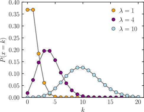
• Poisson distribution PMF example: $p(x) = \frac{e^{-\lambda} \lambda^x}{x!}$ where λ average rate of events

Calculating Probabilities with PMFs

Single and Multiple Outcome Probabilities

• Calculate single outcome probability by evaluating PMF at specific value
• Compute probability for outcome ranges by summing PMF values over desired outcomes
• Example: Fair six-sided die
  • $P(X = 3) = \frac{1}{6}$ (single outcome)
  • $P(X \leq 3) = P(X = 1) + P(X = 2) + P(X = 3) = \frac{1}{6} + \frac{1}{6} + \frac{1}{6} = \frac{1}{2}$ (multiple outcomes)
• Use multiplication for independent events involving multiple random variables
• Apply conditional probability formulas for dependent events

Expected Value and Variance Calculations

• Compute expected value (mean) using PMF $E[X] = \sum_{x} x \cdot p(x)$
• Calculate variance using PMF and expected value $Var(X) = E[(X - E[X])^2] = \sum_{x} (x - E[X])^2 \cdot p(x)$
• Derive standard deviation as square root of variance $\sigma = \sqrt{Var(X)}$
• Example: Expected value for fair six-sided die $E[X] = 1 \cdot \frac{1}{6} + 2 \cdot \frac{1}{6} + 3 \cdot \frac{1}{6} + 4 \cdot \frac{1}{6} + 5 \cdot \frac{1}{6} + 6 \cdot \frac{1}{6} = 3.5$

Constructing PMFs

Methods for PMF Construction

• Identify all possible outcomes of discrete random variable
• Assign non-negative probabilities to each outcome, ensuring sum equals 1
• Express PMF as function, often using piecewise notation for different variable ranges
• Construct empirical PMF from data by calculating relative frequencies of observed outcomes
• Example: Construct PMF for sum of two fair six-sided dice \frac{1}{36} & \text{if } x = 2 \text{ or } x = 12 \\ \frac{2}{36} & \text{if } x = 3 \text{ or } x = 11 \\ \frac{3}{36} & \text{if } x = 4 \text{ or } x = 10 \\ \frac{4}{36} & \text{if } x = 5 \text{ or } x = 9 \\ \frac{5}{36} & \text{if } x = 6 \text{ or } x = 8 \\ \frac{6}{36} & \text{if } x = 7 \end{cases}$$

Verification and Considerations

• Verify constructed PMF satisfies all valid probability mass function properties
• Ensure non-negativity of all probabilities
• Confirm sum of all probabilities equals 1
• Consider underlying distributions informing PMF shape (uniform, normal, exponential)
• Examine symmetry or patterns in data to guide PMF construction
• Example: Verify PMF for sum of two dice $\sum_{x=2}^{12} p(x) = \frac{1}{36} + \frac{2}{36} + \frac{3}{36} + \frac{4}{36} + \frac{5}{36} + \frac{6}{36} + \frac{5}{36} + \frac{4}{36} + \frac{3}{36} + \frac{2}{36} + \frac{1}{36} = 1$

PMFs vs Cumulative Distribution Functions

Relationship and Conversion

• Derive cumulative distribution function (CDF) from PMF by summing probabilities of values less than or equal to given value $F(x) = P(X \leq x) = \sum_{t \leq x} p(t)$
• CDF approaches 1 as random variable increases, non-decreasing function
• Obtain PMF from CDF by taking difference between consecutive CDF values $p(x) = F(x) - F(x-1)$
• Example: CDF for fair coin toss (H = 1, T = 0) 0 & \text{if } x < 0 \\ \frac{1}{2} & \text{if } 0 \leq x < 1 \\ 1 & \text{if } x \geq 1 \end{cases}$$

Characteristics and Applications

• PMF provides probabilities for exact values, CDF for values less than or equal to given value
• CDF continuous from right, including probability of current value
• CDF for discrete random variables step function, jumps occur at PMF support values
• Use CDF to calculate probabilities of ranges efficiently $P(a < X \leq b) = F(b) - F(a)$
• Example: Calculate probability of rolling 3 or less on fair die using CDF $P(X \leq 3) = F(3) = \frac{1}{6} + \frac{1}{6} + \frac{1}{6} = \frac{1}{2}$