10.4 Independence of random variables

Independence of random variables is a crucial concept in probability theory. It occurs when the outcome of one variable doesn't affect the probability of another. This simplifies calculations and allows for easier modeling of complex systems.

Understanding independence is key for many real-world applications. It's used in statistical inference, hypothesis testing, and data analysis. Knowing when variables are independent helps in making accurate predictions and drawing valid conclusions from data.

Independence of Random Variables

Defining Independence

Top images from around the web for Defining Independence

• 

  Conditional probability distribution - Wikipedia View original

  Is this image relevant?

• 

  Distribución marginal - Wikipedia, la enciclopedia libre View original

  Is this image relevant?

• 

  Continuous Probability Functions | Introduction to Statistics View original

  Is this image relevant?

• 

  Conditional probability distribution - Wikipedia View original

  Is this image relevant?

• 

  Distribución marginal - Wikipedia, la enciclopedia libre View original

  Is this image relevant?

1 of 3

Top images from around the web for Defining Independence

• 

  Conditional probability distribution - Wikipedia View original

  Is this image relevant?

• 

  Distribución marginal - Wikipedia, la enciclopedia libre View original

  Is this image relevant?

• 

  Continuous Probability Functions | Introduction to Statistics View original

  Is this image relevant?

• 

  Conditional probability distribution - Wikipedia View original

  Is this image relevant?

• 

  Distribución marginal - Wikipedia, la enciclopedia libre View original

  Is this image relevant?

1 of 3

• Independence between random variables implies occurrence or value of one variable does not affect probability distribution of the other
• Two random variables X and Y considered independent if joint probability distribution expressed as product of marginal distributions: $P(X,Y) = P(X) * P(Y)$
• For discrete random variables, independence means $P(X=x, Y=y) = P(X=x) * P(Y=y)$ for all possible values of x and y
• Continuous random variables characterized by $f(x,y) = f_X(x) * f_Y(y)$, where f(x,y) represents joint probability density function and f_X(x) and f_Y(y) represent marginal density functions
• Independence implies conditional probability of one variable given the other equals its marginal probability: $P(X|Y) = P(X)$ and $P(Y|X) = P(Y)$
• Concept extends to more than two random variables, where mutual independence requires every subset of variables be independent
  • Example: For three random variables X, Y, and Z, mutual independence requires $P(X,Y,Z) = P(X) * P(Y) * P(Z)$, as well as pairwise independence

Practical Implications

• Independence simplifies probability calculations and statistical analysis
• Allows for easier modeling of complex systems by treating components as separate entities
• Crucial in many real-world applications (coin tosses, dice rolls)
• Assumption of independence often used in statistical inference and hypothesis testing
  • Example: In a clinical trial, assuming the outcomes of different patients are independent allows for simpler analysis of treatment effects

Identifying Independent Variables

Examining Joint Distributions

• Analyze joint probability mass function (PMF) or joint probability density function (PDF) of two random variables
• Calculate marginal distributions of each random variable from joint distribution
• Check if joint distribution factorizes into product of marginal distributions for all possible values of random variables
• For discrete random variables, verify $P(X=x, Y=y) = P(X=x) * P(Y=y)$ holds for all x and y in sample space
  • Example: For two fair six-sided dice rolls, $P(X=3, Y=4) = \frac{1}{6} * \frac{1}{6} = \frac{1}{36}$
• For continuous random variables, confirm $f(x,y) = f_X(x) * f_Y(y)$ is true for all x and y in sample space
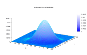
  • Example: Two independent standard normal variables have joint PDF $f(x,y) = \frac{1}{\sqrt{2\pi}} e^{-\frac{x^2}{2}} * \frac{1}{\sqrt{2\pi}} e^{-\frac{y^2}{2}}$

Alternative Methods

• Calculate conditional probabilities and compare them to marginal probabilities to check for independence
• Uncorrelated random variables not necessarily independent, but independent random variables always uncorrelated
• Use covariance or correlation coefficient to test for linear dependence
  • Example: If Cov(X,Y) = 0, X and Y are uncorrelated, but may not be independent
• Examine scatter plots or contingency tables to visually assess potential dependence
  • Example: Random scatter suggests independence, while clear patterns indicate dependence

Multiplicative Rule for Independence

Applying the Rule

• Multiplicative rule for independent events states $P(A \text{ and } B) = P(A) * P(B)$ when A and B are independent
• For independent random variables X and Y, expectation of their product is $E[XY] = E[X] * E[Y]$
• Variance of sum of independent random variables equals sum of their individual variances: $Var(X + Y) = Var(X) + Var(Y)$
• Moment-generating function of sum of independent random variables is product of their individual moment-generating functions
• Probability of sum of independent random variables being less than or equal to value is convolution of their individual distribution functions
  • Example: For independent X ~ N(μ1, σ1^2) and Y ~ N(μ2, σ2^2), X + Y ~ N(μ1 + μ2, σ1^2 + σ2^2)

Problem-Solving Applications

• Independence simplifies calculations in many probability problems, especially those involving multiple random variables or repeated trials
• Apply these principles to solve problems involving independent trials (binomial and Poisson processes)
  • Example: In a binomial distribution, probability of k successes in n independent trials is $P(X=k) = \binom{n}{k} p^k (1-p)^{n-k}$
• Use in reliability analysis to calculate probability of system failure with independent components
  • Example: For a system with two independent components with failure probabilities p1 and p2, probability of system failure is $1 - (1-p1)(1-p2)$

Independence and Distributions

Effects on Marginal and Conditional Distributions

• Marginal distribution of one variable remains unchanged regardless of value of other variable for independent random variables
• Conditional distribution of independent random variable identical to its marginal distribution: $f_{X|Y}(x|y) = f_X(x)$ for all y
• Independence implies knowing value of one variable provides no information about other variable's distribution
• Covariance between independent random variables is zero: $Cov(X,Y) = 0$
• Independence allows for simplified computation of joint moments, as $E[X^n * Y^m] = E[X^n] * E[Y^m]$ for independent X and Y

Applications and Importance

• Central limit theorem relies on assumption of independence when dealing with sum of random variables
• Understanding independence crucial for correctly applying probability models in various fields (statistics, physics, finance)
• Independence assumption often used in statistical hypothesis testing and confidence interval construction
  • Example: In t-tests, samples are assumed to be independent for valid inference
• Important in machine learning and data science for feature selection and model assumptions
  • Example: Naive Bayes classifier assumes independence between features, simplifying probability calculations