7.3 Functions of Matrices and Powers of Matrices

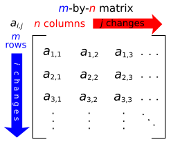
Functions of matrices and powers of matrices are powerful tools in linear algebra. They allow us to extend scalar operations to matrices, opening up new ways to solve complex problems. These concepts are crucial for understanding how matrices behave under various operations.

Diagonalization is key to efficiently computing matrix functions and powers. By breaking down a matrix into simpler components, we can perform calculations more easily and gain insights into the matrix's properties. This connects directly to the broader applications of diagonalization in linear algebra.

Matrix functions through diagonalization

Definition and properties of matrix functions

• A matrix function $f(A)$ is defined for a diagonalizable matrix $A$ as $f(A) = Pf(D)P^{-1}$, where $A = PDP^{-1}$ is the diagonalization of $A$ and $f(D)$ is the diagonal matrix obtained by applying $f$ to each diagonal entry of $D$
• The diagonalization approach allows matrix functions to be computed efficiently and simplifies their properties
• Common matrix functions include the exponential $(e^A)$, logarithm $(\log(A))$, and trigonometric functions $(\sin(A), \cos(A))$
• Properties of matrix functions include:
  • $f(A)f(B) = f(A+B)$ for commuting matrices $A$ and $B$ (e.g., $e^Ae^B = e^{A+B}$ if $AB = BA$)
  • $f(A^T) = (f(A))^T$ (e.g., $(e^A)^T = e^{A^T}$)
  • $f(PAP^{-1}) = Pf(A)P^{-1}$ for invertible $P$ (e.g., $e^{PAP^{-1}} = Pe^AP^{-1}$)

Applications of matrix functions

• Matrix functions have applications in various fields, such as:
  • Solving systems of linear differential equations (e.g., $\frac{d\mathbf{x}}{dt} = A\mathbf{x}$ has solution $\mathbf{x}(t) = e^{At}\mathbf{x}(0)$)
  • Markov processes and stochastic matrices (e.g., the transition matrix after $n$ steps is given by $P^n$)
  • Control theory and state-space models (e.g., the state transition matrix is $e^{At}$)
• Examples of matrix functions in action:
  • The matrix exponential of a skew-symmetric matrix $A$ (i.e., $A^T = -A$) is an orthogonal matrix (i.e., $e^A(e^A)^T = I$)
  • The matrix logarithm can be used to interpolate between two positive definite matrices $A$ and $B$ using the geodesic path $A(t) = A^{1-t}B^t = A\exp(t\log(A^{-1}B))$

Efficient power calculations for matrices

Diagonalization for computing matrix powers

• For a diagonalizable matrix $A = PDP^{-1}$, the $k$-th power of $A$ can be computed as $A^k = PD^kP^{-1}$, where $D^k$ is obtained by raising each diagonal entry of $D$ to the $k$-th power
• This method is more efficient than directly multiplying $A$ by itself $k$ times, especially for large matrices or high powers
• Negative integer powers can be computed using the inverse: $A^{-k} = (A^{-1})^k = PD^{-k}P^{-1}$
• Fractional powers can be computed by taking the appropriate roots of the diagonal entries: $A^{1/k} = PD^{1/k}P^{-1}$

Examples and applications of matrix powers

• Computing the $n$-th Fibonacci number using the matrix power method:
  • Define $A = \begin{pmatrix} 1 & 1 \\ 1 & 0 \end{pmatrix}$, then $A^n = \begin{pmatrix} F_{n+1} & F_n \\ F_n & F_{n-1} \end{pmatrix}$, where $F_n$ is the $n$-th Fibonacci number
  • Diagonalization of $A$ allows for efficient computation of $A^n$ and, consequently, $F_n$
• Analyzing the long-term behavior of a Markov chain:
  • The steady-state distribution of a regular Markov chain with transition matrix $P$ is given by the normalized left eigenvector of $P$ corresponding to the eigenvalue 1
  • Powers of $P$ converge to a matrix with identical rows equal to the steady-state distribution

Diagonalization for matrix exponentials and logarithms

Computing matrix exponentials and logarithms

• The matrix exponential is defined as $e^A = Pe^DP^{-1}$, where $e^D$ is the diagonal matrix obtained by applying the scalar exponential function to each diagonal entry of $D$
• The matrix logarithm is the inverse function of the matrix exponential: if $e^A = B$, then $\log(B) = A$. It is defined only for invertible matrices with no negative real eigenvalues
• Properties of matrix exponentials include:
  • $e^{A+B} = e^Ae^B$ for commuting matrices $A$ and $B$
  • $(e^A)^T = e^{A^T}$
  • $e^{PAP^{-1}} = Pe^AP^{-1}$ for invertible $P$

Applications of matrix exponentials and logarithms

• Matrix exponentials and logarithms have applications in solving systems of linear differential equations, Markov processes, and control theory
• Examples of matrix exponentials and logarithms in action:
  • The solution to the first-order linear differential equation $\frac{d\mathbf{x}}{dt} = A\mathbf{x}$ with initial condition $\mathbf{x}(0) = \mathbf{x}_0$ is given by $\mathbf{x}(t) = e^{At}\mathbf{x}_0$
  • The matrix logarithm can be used to compute the principal logarithm of a complex number $z = re^{i\theta}$ using the matrix identity $\log(z) = \log(r) + i\theta = \log\left(\begin{pmatrix} r & 0 \\ 0 & r \end{pmatrix}\right) + \log\left(\begin{pmatrix} \cos\theta & -\sin\theta \\ \sin\theta & \cos\theta \end{pmatrix}\right)$

Solving matrix equations with functions

Techniques for solving matrix equations involving functions

• Matrix equations involving functions of matrices, such as $e^AX - Xe^B = C$ or $A\log(X) + \log(X)B = C$, can often be solved using diagonalization
• If $A$ and $B$ are diagonalizable with eigenvalue matrices $D_A$ and $D_B$, respectively, the equation $e^AX - Xe^B = C$ can be transformed into $e^{D_A}Y - Ye^{D_B} = P_A^{-1}CP_B$, where $X = P_AYP_B^{-1}$. This transformed equation can be solved for $Y$, and then $X$ can be obtained by reversing the transformation
• Similarly, for the equation $A\log(X) + \log(X)B = C$, diagonalization can be used to transform it into $D_AZ + ZD_B = P_A^{-1}CP_B$, where $\log(X) = P_AZP_B^{-1}$. Solve for $Z$ and then obtain $\log(X)$ and, subsequently, $X$
• In some cases, additional techniques such as vectorization or the Kronecker product may be needed to solve the transformed equations

Examples of solving matrix equations with functions

• Solving the matrix equation $e^AX - Xe^B = C$:
  • Diagonalize $A = P_AD_AP_A^{-1}$ and $B = P_BD_BP_B^{-1}$
  • Transform the equation to $e^{D_A}Y - Ye^{D_B} = P_A^{-1}CP_B$, where $X = P_AYP_B^{-1}$
  • Solve the transformed equation for $Y$ by equating corresponding entries
  • Obtain the solution $X = P_AYP_B^{-1}$
• Solving the matrix equation $A\log(X) + \log(X)B = C$:
  • Diagonalize $A = P_AD_AP_A^{-1}$ and $B = P_BD_BP_B^{-1}$
  • Transform the equation to $D_AZ + ZD_B = P_A^{-1}CP_B$, where $\log(X) = P_AZP_B^{-1}$
  • Solve the transformed equation for $Z$ by equating corresponding entries
  • Obtain $\log(X) = P_AZP_B^{-1}$ and then compute $X = e^{\log(X)}$