5.3 Chapman-Kolmogorov equations

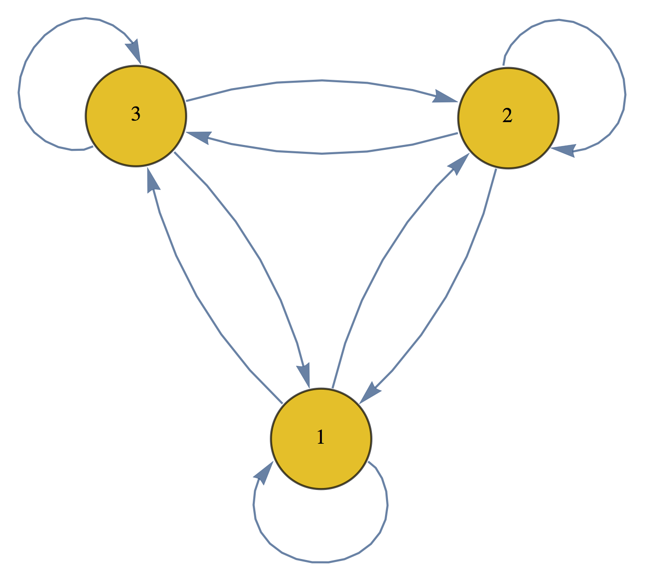
Definition of Chapman-Kolmogorov equations

The Chapman-Kolmogorov (C-K) equations express a simple but powerful idea: to find the probability of going from state $i$ to state $j$ in $m + n$ steps, you can break that journey at any intermediate time and sum over all possible intermediate states $k$. This works because of the Markov property (only the current state matters, not how you got there) combined with the law of total probability.

These equations are fundamental for computing n-step transition probabilities and, ultimately, steady-state distributions. They apply to both discrete-time and continuous-time Markov chains.

Derivation of the equations

Start with a Markov chain on a finite or countable state space. Let $p_{ij}^{(n)} = P(X_n = j \mid X_0 = i)$ denote the probability of transitioning from state $i$ to state $j$ in $n$ steps.

The derivation proceeds as follows:

1. Pick any intermediate time $m$ with $0 \leq m \leq m+n$.
2. By the law of total probability, condition on the state $k$ occupied at time $m$: $P(X_{m+n} = j \mid X_0 = i) = \sum_k P(X_m = k \mid X_0 = i) \cdot P(X_{m+n} = j \mid X_m = k)$
3. Apply the Markov property: given $X_m = k$, the future evolution doesn't depend on how the chain reached $k$. So $P(X_{m+n} = j \mid X_m = k) = P(X_n = j \mid X_0 = k)$ (assuming time-homogeneity).
4. This gives the Chapman-Kolmogorov equation: $p_{ij}^{(m+n)} = \sum_k p_{ik}^{(m)} \cdot p_{kj}^{(n)}$

The entire argument rests on two ingredients: the Markov property (memorylessness) and the law of total probability (partitioning over intermediate states).

Discrete-time Markov chains

A discrete-time Markov chain (DTMC) has a discrete state space and evolves at integer time steps. It's fully characterized by its transition probability matrix $P$, where entry $p_{ij}$ is the one-step probability of moving from state $i$ to state $j$.

State transition probabilities

The entries of $P$ must satisfy two properties:

• $p_{ij} \geq 0$ for all $i, j$ (probabilities are non-negative)
• $\sum_j p_{ij} = 1$ for all $i$ (each row sums to 1, since the chain must go somewhere)

In this setting, the C-K equations take the form:

$p_{ij}^{(m+n)} = \sum_k p_{ik}^{(m)} \cdot p_{kj}^{(n)}$

Notice that the right-hand side is exactly the $(i,j)$ entry of the matrix product $P^{(m)} \cdot P^{(n)}$. This connects the probabilistic statement directly to matrix multiplication.

n-step transition probabilities

Because the C-K equations correspond to matrix multiplication, computing the $n$-step transition matrix is straightforward:

$P^{(n)} = P^n$

You raise the one-step matrix $P$ to the $n$th power. For small $n$, you can do this directly. For large $n$, the C-K equations let you split the computation efficiently. For example, $P^{(8)} = P^{(4)} \cdot P^{(4)}$, so you only need to compute $P^{(4)}$ and square it (this is the idea behind exponentiation by squaring).

The steady-state distribution $\pi$ satisfies $\pi P = \pi$ along with $\sum_j \pi_j = 1$. It describes the long-run fraction of time the chain spends in each state. You find it by solving this system of linear equations. The C-K equations are what justify looking at $P^n$ as $n \to \infty$ to study convergence to $\pi$.

Continuous-time Markov chains

A continuous-time Markov chain (CTMC) has a discrete state space but transitions can occur at any point in continuous time. Instead of a transition probability matrix, a CTMC is characterized by a transition rate matrix (or generator matrix) $Q$, where $q_{ij}$ (for $i \neq j$) is the rate of transitioning from state $i$ to state $j$, and $q_{ii} = -\sum_{j \neq i} q_{ij}$.

Transition probability functions

The transition probability function $P(t)$ gives the matrix of probabilities $p_{ij}(t) = P(X(t+s) = j \mid X(s) = i)$ for transitioning between states over a time interval of length $t$.

The C-K equations in continuous time take the matrix form:

$P(t + s) = P(t) \cdot P(s) \quad \text{for any } t, s \geq 0$

This is the continuous-time analog of $P^{(m+n)} = P^{(m)} \cdot P^{(n)}$. The relationship between $P(t)$ and the rate matrix $Q$ is made precise by the Kolmogorov differential equations.

Kolmogorov forward equations

The forward equations describe how $P(t)$ evolves by looking "forward" from the current time:

$\frac{d}{dt} P(t) = P(t) \cdot Q$

You can read this as: the rate of change of the transition probabilities equals the current probabilities multiplied by the transition rates. Solving this ODE (with initial condition $P(0) = I$) yields $P(t)$.

Kolmogorov backward equations

The backward equations take the opposite perspective, conditioning on what happens at the start of the interval:

$\frac{d}{dt} P(t) = Q \cdot P(t)$

Note the order of multiplication is reversed compared to the forward equations. Both equations have the same solution $P(t) = e^{tQ}$, but they arise from different conditioning arguments. In practice, the forward equations are more commonly used for computing state probabilities, while the backward equations appear more often in theoretical work and certain first-passage-time problems.

Applications of Chapman-Kolmogorov equations

Queueing theory

Queueing models (for customer service centers, network routers, etc.) use Markov chains to represent the number of customers in the system. The C-K equations let you compute performance measures like average queue length, waiting time distributions, and server utilization by finding transient or steady-state probabilities of the underlying chain.

Birth-death processes

In a birth-death process, the state represents a population count, and transitions only occur between neighboring states (the population increases or decreases by one). Birth and death rates define the generator matrix $Q$. The C-K equations enable computation of both transient probabilities (how the population distribution evolves over time) and steady-state probabilities (the long-run population distribution).

Reliability analysis

For systems like power grids or manufacturing plants, components fail and get repaired over time. A Markov chain tracks the system's operational state. The C-K equations help calculate reliability metrics such as mean time to failure (MTTF), availability (fraction of time the system is operational), and mean time between failures (MTBF).

Relationship to other concepts

Markov property

The C-K equations are a direct consequence of the Markov property. Without memorylessness, you couldn't factor the multi-step transition probability into a product of shorter-step probabilities summed over intermediate states. If the process had memory, the probability of reaching $j$ from $k$ would depend on how the chain arrived at $k$, and the decomposition would fail.

Stationarity (time-homogeneity)

A Markov chain is time-homogeneous (or has stationary transition probabilities) if $P(X_{n+1} = j \mid X_n = i)$ doesn't depend on $n$. Under time-homogeneity, the C-K equations simplify because $p_{ij}^{(n)}$ depends only on the number of steps $n$, not on when those steps occur. This is the standard setting assumed throughout most of this guide.

Ergodicity

An ergodic Markov chain is one that is irreducible (every state can be reached from every other state) and aperiodic (the chain doesn't cycle with a fixed period). Ergodicity guarantees a unique steady-state distribution $\pi$ that the chain converges to regardless of the initial state. The C-K equations, through $P^n$ as $n \to \infty$, are the mechanism by which you verify and compute this convergence.

Numerical methods for solving the equations

For chains with large state spaces, computing transition probabilities analytically becomes impractical. Two common numerical approaches are outlined below.

Matrix exponential approach

For CTMCs, the solution to the Kolmogorov equations is:

$P(t) = e^{tQ}$

Computing the matrix exponential directly is nontrivial for large matrices. Common numerical methods include:

• Scaling and squaring: Scale $tQ$ down so the exponential is easy to approximate (e.g., via a truncated Taylor series), then repeatedly square the result to recover $e^{tQ}$.
• Padé approximation: Approximate $e^{tQ}$ using a rational function (ratio of polynomials), which often converges faster than a Taylor series.
• Uniformization (Jensen's method): Convert the CTMC into an equivalent DTMC by choosing a uniform transition rate, then compute a weighted Poisson sum of matrix powers. This is numerically stable and widely used.

Eigenvalue decomposition

For a DTMC, if $P$ is diagonalizable, you can write:

$P = V \Lambda V^{-1}$

where $V$ is the matrix of eigenvectors and $\Lambda$ is the diagonal matrix of eigenvalues. Then:

$P^{(n)} = P^n = V \Lambda^n V^{-1}$

Raising a diagonal matrix to the $n$th power just means raising each eigenvalue to the $n$th power, which is trivial. This approach is especially efficient for large $n$ because the cost of the eigendecomposition is paid once, and then any $P^n$ is cheap to compute. It also gives direct insight into convergence rates: the second-largest eigenvalue magnitude controls how fast the chain approaches its steady state.

Extensions and generalizations

Semi-Markov processes

Standard CTMCs require exponentially distributed holding times in each state. Semi-Markov processes relax this by allowing arbitrary holding time distributions (e.g., Weibull, log-normal). The C-K equations generalize to involve convolutions of holding time distributions with transition probabilities, making the analysis more complex but also more realistic for systems where the exponential assumption is too restrictive.

Non-homogeneous Markov chains

When transition probabilities change over time (due to seasonal effects, aging, policy changes, etc.), the chain is non-homogeneous. The C-K equations still hold, but now involve time-dependent transition matrices:

$P(s, s+t) = P(s, s+u) \cdot P(s+u, s+t) \quad \text{for } 0 \leq u \leq t$

Here $P(s, t)$ denotes the transition matrix from time $s$ to time $t$. You can no longer simply raise a single matrix to a power; instead, you must multiply a sequence of different matrices.

Markov renewal processes

These generalize semi-Markov processes by jointly modeling the next state visited and the time until the next transition through a renewal kernel. The C-K equations become renewal equations relating transition probabilities to the kernel. Markov renewal theory provides a unified framework that includes ordinary renewal processes, DTMCs, CTMCs, and semi-Markov processes as special cases.