6.4 Stationary distributions

Definition of Stationary Distributions

A stationary distribution for a continuous-time Markov chain (CTMC) is a probability distribution over the state space that remains unchanged as the process evolves. If the chain is "in" its stationary distribution at some moment, it stays in that distribution for all future times.

Formally, a probability vector $\pi$ is stationary for a CTMC with generator matrix $Q$ if it satisfies:

$\pi Q = 0, \quad \sum_i \pi_i = 1, \quad \pi_i \geq 0 \text{ for all } i$

The equation $\pi Q = 0$ is the continuous-time analogue of $\pi P = \pi$ in discrete time. Because the generator $Q$ encodes transition rates rather than transition probabilities, the stationarity condition takes this slightly different form.

Existence and Uniqueness

Whether a CTMC has a stationary distribution depends on structural properties of the chain:

• Irreducibility: Every state can be reached from every other state. There's a path of positive-rate transitions connecting any pair of states.
• Positive recurrence: Starting from any state, the expected time to return to that state is finite. For finite-state irreducible chains, positive recurrence is automatic.

If a CTMC is irreducible and positive recurrent, it has a unique stationary distribution. For finite irreducible chains, this is always guaranteed.

A reducible chain can have multiple stationary distributions (one for each closed communicating class, and convex combinations of these). A chain that is irreducible but not positive recurrent (null recurrent or transient) has no stationary distribution.

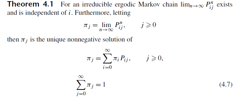
Relationship to Limiting Distributions

The limiting distribution describes where the chain ends up as $t \to \infty$, regardless of where it started. Specifically, $\lim_{t \to \infty} P_{ij}(t)$ gives the limiting probability of being in state $j$.

For CTMCs, the relationship is cleaner than in discrete time because there's no periodicity issue (continuous-time chains are inherently aperiodic). If a CTMC is irreducible and positive recurrent, the limiting distribution exists and equals the unique stationary distribution:

$\lim_{t \to \infty} P_{ij}(t) = \pi_j \quad \text{for all } i, j$

So for well-behaved CTMCs, the stationary distribution is the limiting distribution. The distinction matters more in discrete time, where periodicity can prevent convergence to a limit even when a stationary distribution exists.

Computation Methods

Global Balance Equations

The global balance equations state that, for each state $i$, the total rate of probability flow out of $i$ equals the total rate of flow into $i$:

$\pi_i \sum_{j \neq i} q_{ij} = \sum_{j \neq i} \pi_j \, q_{ji}$

Here $q_{ij}$ is the rate of transitioning from state $i$ to state $j$ (the off-diagonal entries of $Q$).

To find $\pi$:

1. Write out the global balance equation for each state.
2. Note that these equations are linearly dependent (they all encode $\pi Q = 0$), so drop one equation.
3. Replace the dropped equation with the normalization condition $\sum_i \pi_i = 1$.
4. Solve the resulting system of linear equations.

Detailed Balance (Reversibility)

For many chains encountered in practice, a stronger condition called detailed balance holds:

$\pi_i \, q_{ij} = \pi_j \, q_{ji} \quad \text{for all } i \neq j$

This says the rate of flow from $i$ to $j$ equals the rate from $j$ to $i$, pairwise. Detailed balance implies global balance (sum both sides over $j$), but not vice versa.

When detailed balance holds, the chain is called reversible, and finding $\pi$ is often much easier because you can solve the pairwise equations directly rather than dealing with the full system.

Using the Embedded Chain

Another approach connects the CTMC to its embedded discrete-time chain. If $\tilde{\pi}$ is the stationary distribution of the embedded chain (with transition probabilities $p_{ij} = q_{ij}/q_i$ where $q_i = \sum_{j \neq i} q_{ij}$), then the CTMC stationary distribution is:

$\pi_i = \frac{\tilde{\pi}_i / q_i}{\sum_k \tilde{\pi}_k / q_k}$

This formula weights each state by the reciprocal of its total departure rate $q_i$, reflecting the fact that the chain spends more time in states it leaves slowly.

Properties

Invariance

If you initialize a CTMC according to $\pi$, then at every future time $t > 0$ the distribution over states is still $\pi$. This is the defining property, and it follows directly from $\pi Q = 0$ (equivalently, $\pi P(t) = \pi$ for all $t \geq 0$, where $P(t) = e^{Qt}$ is the transition semigroup).

Long-Run Time Averages

The entries of $\pi$ have a concrete interpretation: $\pi_i$ equals the long-run fraction of time the chain spends in state $i$. More precisely, for an irreducible positive-recurrent CTMC:

$\pi_i = \lim_{T \to \infty} \frac{1}{T} \int_0^T \mathbf{1}\{X(s) = i\} \, ds \quad \text{(with probability 1)}$

This holds regardless of the initial state. It also means $\pi_i = 1 / (q_i \cdot E_i[T_i])$ where $E_i[T_i]$ is the expected return time to state $i$ (counting both holding times and transitions).

Relationship to Mean Holding Times

Because a CTMC holds in state $i$ for an exponential time with rate $q_i$, states with smaller $q_i$ (slower departure rates) tend to have larger stationary probabilities. The embedded-chain formula above makes this precise.

Examples

Birth-Death Processes

Birth-death CTMCs have states $\{0, 1, 2, \ldots\}$ with only nearest-neighbor transitions: birth rate $\lambda_n$ (from $n$ to $n+1$) and death rate $\mu_n$ (from $n$ to $n-1$).

Detailed balance holds automatically for birth-death chains, giving:

$\pi_n \lambda_n = \pi_{n+1} \mu_{n+1}$

Solving recursively:

$\pi_n = \pi_0 \prod_{k=0}^{n-1} \frac{\lambda_k}{\mu_{k+1}}$

Then $\pi_0$ is determined by normalization: $\sum_{n=0}^{\infty} \pi_n = 1$. A stationary distribution exists if and only if this sum converges.

For example, with constant rates $\lambda_n = \lambda$ and $\mu_n = \mu$, the ratio is $\rho = \lambda/\mu$, and convergence requires $\rho < 1$.

Random Walks

A continuous-time random walk on a finite graph assigns jump rates to each edge. On a finite connected graph with symmetric rates ($q_{ij} = q_{ji}$), detailed balance is satisfied and the stationary distribution is proportional to $1/q_i$ (where $q_i$ is the total rate out of state $i$). If all rates are equal, this gives a uniform stationary distribution.

Queueing Models

The M/M/1 queue has Poisson arrivals at rate $\lambda$ and exponential service at rate $\mu$. This is a birth-death process with constant rates, so the stationary distribution (when $\rho = \lambda/\mu < 1$) is geometric:

$\pi_n = (1 - \rho)\rho^n, \quad n = 0, 1, 2, \ldots$

From this you can derive performance measures like the expected number of customers ($E[N] = \rho/(1-\rho)$) and the expected time in the system ($E[T] = 1/(\mu - \lambda)$ by Little's law).

The M/M/c queue ($c$ servers) has a similar structure but with state-dependent service rates: $\mu_n = \min(n, c) \cdot \mu$. The stationary distribution involves an Erlang-C formula, and stability requires $\lambda < c\mu$.

Applications

Steady-State Performance Analysis

In practice, you often care about long-run averages: the mean queue length, the fraction of time a server is idle, the throughput of a network. The stationary distribution gives you all of these directly. Once you have $\pi$, any steady-state quantity is just a weighted sum $\sum_i f(i)\pi_i$ for the appropriate function $f$.

Ergodicity and Convergence

A CTMC is ergodic if it's irreducible and positive recurrent. Ergodicity guarantees:

• A unique stationary distribution exists.
• The chain converges to it from any starting state.
• Time averages equal ensemble averages (the ergodic theorem).

This is what justifies using stationary distributions in practice. You don't need to know the initial state to predict long-run behavior.

Simulation and MCMC

Markov chain Monte Carlo (MCMC) methods construct a Markov chain whose stationary distribution is a target distribution you want to sample from. The Metropolis-Hastings algorithm and Gibbs sampler are the most common examples. After running the chain long enough to approximately reach stationarity (the "burn-in" period), subsequent samples approximate draws from the target distribution.

Stationary Distributions vs. Limiting Distributions

For CTMCs, these two concepts coincide whenever the chain is irreducible and positive recurrent. The lack of periodicity in continuous time simplifies things compared to the discrete-time case, where a periodic chain can have a stationary distribution but no limiting distribution.

A chain that is not positive recurrent (e.g., a symmetric random walk on $\mathbb{Z}$) has neither a stationary nor a limiting distribution.

Extensions

Quasi-Stationary Distributions

When a CTMC has absorbing states (states it can enter but never leave), the chain will eventually be absorbed with probability 1. A quasi-stationary distribution describes the conditional distribution over transient states, given that absorption hasn't happened yet:

$\lim_{t \to \infty} P(X(t) = i \mid X(t) \notin A) = \nu_i$

where $A$ is the set of absorbing states. This is useful in population models (where extinction is the absorbing state) and reliability theory (where system failure is absorbing).

Stationary Distributions for General CTMCs

For CTMCs on countably infinite state spaces, existence of a stationary distribution is not guaranteed even for irreducible chains. The chain must be positive recurrent. Standard tools for verifying positive recurrence include:

• Foster-Lyapunov criteria: Find a function $V$ on the state space such that $QV(i) \leq -\epsilon$ outside a finite set, which implies positive recurrence.
• Direct computation: For birth-death chains, check whether $\sum_n \pi_n < \infty$ using the product-form solution.