1.6 Moment-generating functions

Definition of moment-generating functions

The moment-generating function (MGF) of a random variable $X$ is defined as:

$M_X(t) = E[e^{tX}]$

where $t$ is a real number. The name comes from what this function does: it generates the moments of a distribution (mean, variance, skewness, kurtosis) through differentiation. MGFs also uniquely characterize distributions, making them one of the most versatile tools in probability theory.

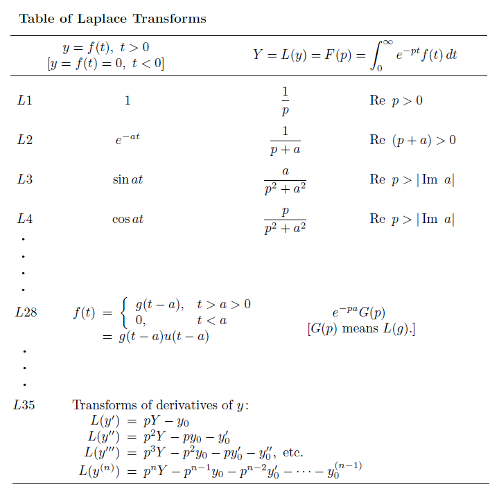
Laplace transforms vs moment-generating functions

MGFs are closely related to Laplace transforms, which show up heavily in engineering and physics for solving differential equations. The two-sided Laplace transform of a probability density is $E[e^{-sX}]$, so the MGF is simply the Laplace transform evaluated at $s = -t$. In practice, Laplace transforms typically deal with functions defined on $[0, \infty)$, while MGFs apply to random variables on the entire real line.

Existence of moment-generating functions

Not every distribution has a valid MGF. For $M_X(t)$ to exist, the expectation $E[e^{tX}]$ must be finite for all $t$ in some open interval around zero (i.e., for $t \in (-h, h)$ with $h > 0$).

Distributions with heavy tails can violate this condition. The Cauchy distribution is the classic example: its tails decay so slowly that $E[e^{tX}]$ diverges for every $t \neq 0$. When an MGF doesn't exist, the characteristic function (which uses $E[e^{itX}]$ with $i = \sqrt{-1}$) serves as an alternative that always exists.

Uniqueness of distributions and moment-generating functions

If two random variables have MGFs that are equal on some open interval containing zero, then they have the same distribution. This uniqueness theorem is what makes MGFs so useful for identifying distributions and proving distributional results.

Note that the converse concern sometimes raised about "two different MGFs corresponding to the same distribution" is not actually an issue: if two random variables share the same distribution, their MGFs are necessarily identical wherever they exist. The uniqueness runs in both directions.

Properties of moment-generating functions

Derivatives and moment extraction

This is the core property that gives MGFs their name. The $n$-th moment of $X$ equals the $n$-th derivative of $M_X(t)$ evaluated at $t = 0$:

$E[X^n] = M_X^{(n)}(0)$

Why does this work? Expand $e^{tX}$ as a Taylor series:

$M_X(t) = E[e^{tX}] = E\left[\sum_{n=0}^{\infty} \frac{(tX)^n}{n!}\right] = \sum_{n=0}^{\infty} \frac{E[X^n]}{n!} \, t^n$

Each coefficient encodes a moment. Differentiating $n$ times and setting $t = 0$ isolates $E[X^n]$.

In practice, the most common extractions are:

• Mean: $E[X] = M_X'(0)$
• Variance: $\text{Var}(X) = M_X''(0) - \left(M_X'(0)\right)^2$
• Higher moments (skewness, kurtosis) follow from higher-order derivatives.

Linear transformations

For a random variable $Y = aX + b$, the MGF transforms as:

$M_Y(t) = e^{bt} \, M_X(at)$

This follows directly from the definition: $E[e^{t(aX+b)}] = e^{bt} \, E[e^{(at)X}]$.

Sums of independent random variables

For independent random variables $X$ and $Y$, the MGF of their sum factors into a product:

$M_{X+Y}(t) = M_X(t) \cdot M_Y(t)$

This extends to any finite collection. If $X_1, X_2, \ldots, X_n$ are independent:

$M_{X_1 + X_2 + \cdots + X_n}(t) = \prod_{i=1}^{n} M_{X_i}(t)$

The factoring happens because independence lets you split the joint expectation: $E[e^{t(X+Y)}] = E[e^{tX}] \cdot E[e^{tY}]$. This property is what makes MGFs so effective for working with sums.

Moment-generating functions of common distributions

Discrete distributions

• Bernoulli (parameter $p$): $M_X(t) = 1 - p + pe^t$
• Binomial (parameters $n, p$): $M_X(t) = (1 - p + pe^t)^n$
• Poisson (parameter $\lambda$): $M_X(t) = e^{\lambda(e^t - 1)}$
• Geometric (parameter $p$, counting from 1): $M_X(t) = \frac{pe^t}{1 - (1-p)e^t}$ for $t < -\ln(1-p)$

Continuous distributions

• Exponential (rate $\lambda$): $M_X(t) = \frac{\lambda}{\lambda - t}$ for $t < \lambda$
• Normal (mean $\mu$, variance $\sigma^2$): $M_X(t) = e^{\mu t + \frac{1}{2}\sigma^2 t^2}$
• Gamma (shape $\alpha$, rate $\beta$): $M_X(t) = \left(\frac{\beta}{\beta - t}\right)^\alpha$ for $t < \beta$

Worked examples

Example 1: Deriving the standard normal MGF

For $X \sim N(0,1)$:

$M_X(t) = \int_{-\infty}^{\infty} \frac{1}{\sqrt{2\pi}} e^{-x^2/2} \, e^{tx} \, dx = \int_{-\infty}^{\infty} \frac{1}{\sqrt{2\pi}} e^{-(x^2 - 2tx)/2} \, dx$

Complete the square in the exponent: $x^2 - 2tx = (x - t)^2 - t^2$. This gives:

$M_X(t) = e^{t^2/2} \int_{-\infty}^{\infty} \frac{1}{\sqrt{2\pi}} e^{-(x-t)^2/2} \, dx = e^{t^2/2}$

The integral equals 1 because the integrand is the density of a $N(t, 1)$ distribution.

Example 2: Moments of the exponential distribution

For $X \sim \text{Exp}(\lambda)$ with $M_X(t) = \frac{\lambda}{\lambda - t}$:

1. First derivative: $M_X'(t) = \frac{\lambda}{(\lambda - t)^2}$, so $E[X] = M_X'(0) = \frac{1}{\lambda}$

2. Second derivative: $M_X''(t) = \frac{2\lambda}{(\lambda - t)^3}$, so $E[X^2] = M_X''(0) = \frac{2}{\lambda^2}$

3. Variance: $\text{Var}(X) = \frac{2}{\lambda^2} - \left(\frac{1}{\lambda}\right)^2 = \frac{1}{\lambda^2}$

Applications of moment-generating functions

Determining distributions of sums

The product property for independent sums, combined with uniqueness, gives you a clean strategy for identifying the distribution of a sum:

1. Compute the MGF of each independent summand.
2. Multiply them together.
3. Recognize the resulting MGF as belonging to a known distribution.

Example: Let $X_1 \sim \text{Poisson}(\lambda_1)$ and $X_2 \sim \text{Poisson}(\lambda_2)$ be independent. Then:

$M_{X_1 + X_2}(t) = e^{\lambda_1(e^t - 1)} \cdot e^{\lambda_2(e^t - 1)} = e^{(\lambda_1 + \lambda_2)(e^t - 1)}$

This is the MGF of a $\text{Poisson}(\lambda_1 + \lambda_2)$ distribution. By uniqueness, $X_1 + X_2 \sim \text{Poisson}(\lambda_1 + \lambda_2)$.

The same technique works for showing that sums of independent normals are normal, sums of independent gammas (with the same rate) are gamma, and so on.

Role in limit theorems

MGFs provide one of the cleanest routes to proving the Central Limit Theorem (CLT). The argument proceeds roughly as follows:

1. Let $X_1, X_2, \ldots, X_n$ be i.i.d. with mean $\mu$, variance $\sigma^2$, and a valid MGF.

2. Form the standardized sum $Z_n = \frac{\sum X_i - n\mu}{\sigma\sqrt{n}}$.

3. Show that $M_{Z_n}(t) \to e^{t^2/2}$ as $n \to \infty$.

4. Since $e^{t^2/2}$ is the MGF of the standard normal, a continuity theorem guarantees $Z_n \xrightarrow{d} N(0,1)$.

The key step uses a Taylor expansion of $\ln M_X(t)$ around $t = 0$. This MGF-based proof requires the MGF to exist in a neighborhood of zero, which is a stronger condition than the CLT actually needs, but it makes the argument especially transparent.

Characterizing distributions

Because MGFs uniquely determine distributions, you can use them as a fingerprint. If you derive the MGF of some random variable and it matches a known form, you've identified the distribution without needing to work out the full density or PMF. This is often far easier than computing convolutions or transformations directly.