8.4 Conjugate gradient method

The conjugate gradient method is a powerful iterative technique for solving large, sparse linear systems. It's particularly effective for symmetric positive definite matrices, common in scientific and engineering applications. This method minimizes a quadratic function to find solutions efficiently.

Conjugate gradient builds on concepts from linear algebra and optimization theory. It uses conjugate vectors and Gram-Schmidt orthogonalization to create efficient search directions, ensuring rapid convergence for certain matrix types. This approach transforms linear system solving into a minimization problem.

Fundamentals of conjugate gradient

• Iterative method for solving large, sparse systems of linear equations efficiently
• Belongs to the family of Krylov subspace methods, optimizing solution search within specific vector spaces
• Particularly effective for symmetric positive definite matrices, common in various scientific and engineering applications

Definition and purpose

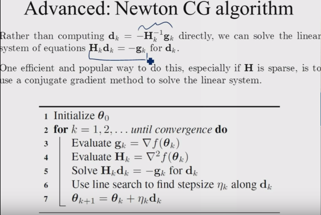
• Numerical algorithm designed to solve $Ax = b$ where A is a symmetric positive definite matrix
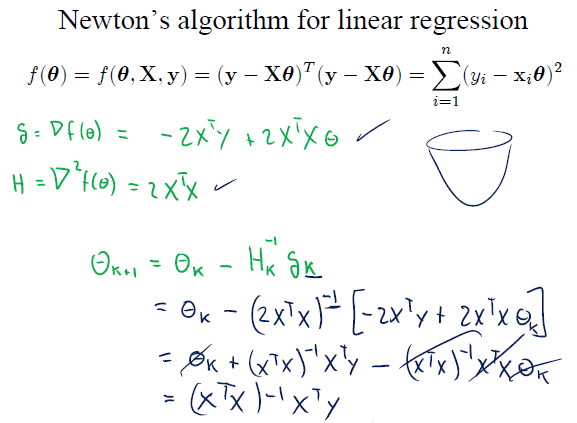
• Minimizes a quadratic function $f(x) = \frac{1}{2}x^TAx - b^Tx + c$ to find the solution
• Generates a sequence of approximate solutions that converge to the exact solution
• Utilizes conjugate directions to improve convergence rate compared to simpler methods (steepest descent)

Historical development

• Introduced by Magnus Hestenes and Eduard Stiefel in 1952
• Originally developed as a direct method for solving linear systems
• Later recognized as an iterative method with superior convergence properties
• Gained popularity in the 1970s with the advent of finite element methods and increased computing power

Relationship to linear systems

• Transforms the problem of solving $Ax = b$ into minimizing a quadratic function
• Exploits the symmetry and positive definiteness of A to generate orthogonal search directions
• Guarantees convergence in at most n iterations for an n x n matrix in exact arithmetic
• Provides an efficient alternative to direct methods (Gaussian elimination) for large, sparse systems

Mathematical foundations

• Builds upon concepts from linear algebra and optimization theory
• Utilizes properties of inner products and vector spaces to construct efficient search directions
• Incorporates ideas from steepest descent methods while improving convergence characteristics

Conjugacy of vectors

• Two vectors u and v are conjugate with respect to A if $u^TAv = 0$
• Conjugate vectors form a basis for the solution space
• Allows for efficient updates of the solution estimate in each iteration
• Ensures that progress made in one direction is not undone by subsequent iterations

Gram-Schmidt orthogonalization

• Process used to generate a set of orthogonal vectors from a given set of linearly independent vectors
• Applied implicitly in the conjugate gradient method to create conjugate search directions
• Maintains orthogonality of residuals and search directions throughout the iterative process
• Enables efficient computation of optimal step sizes in each iteration

Krylov subspace methods

• Family of iterative methods that approximate the solution within Krylov subspaces
• Krylov subspace defined as $K_k(A, r_0) = span\{r_0, Ar_0, A^2r_0, ..., A^{k-1}r_0\}$
• Conjugate gradient method constructs an orthogonal basis for the Krylov subspace
• Exploits the structure of the Krylov subspace to achieve rapid convergence for certain matrix types

Algorithm structure

• Consists of a series of steps that iteratively refine the solution estimate
• Maintains and updates several vectors throughout the process (residual, search direction, solution)
• Computes optimal step sizes to minimize the error in each iteration

Initialization steps

• Set initial guess $x_0$ (often the zero vector)
• Compute initial residual $r_0 = b - Ax_0$
• Set initial search direction $p_0 = r_0$
• Initialize iteration counter k = 0

Iterative process

• Compute step size $\alpha_k = \frac{r_k^T r_k}{p_k^T A p_k}$
• Update solution $x_{k+1} = x_k + \alpha_k p_k$
• Update residual $r_{k+1} = r_k - \alpha_k A p_k$
• Compute beta $\beta_k = \frac{r_{k+1}^T r_{k+1}}{r_k^T r_k}$
• Update search direction $p_{k+1} = r_{k+1} + \beta_k p_k$
• Increment k and repeat until convergence

Convergence criteria

• Monitor the norm of the residual $\|r_k\|$ or relative residual $\frac{\|r_k\|}{\|b\|}$
• Check if the residual falls below a specified tolerance ($\epsilon$)
• Consider the maximum number of iterations as a secondary stopping criterion
• Evaluate the relative change in the solution between consecutive iterations

Computational aspects

• Focuses on efficient implementation and practical considerations
• Addresses challenges related to finite precision arithmetic and large-scale problems
• Incorporates techniques to improve performance and robustness

Matrix-free implementation

• Avoids explicit storage of matrix A, requiring only matrix-vector products
• Enables application to problems where A is defined implicitly or as an operator
• Reduces memory requirements for large-scale systems
• Allows for efficient implementation of matrix-vector products in specialized applications (finite element methods)

Preconditioning techniques

• Transforms the original system to improve convergence properties
• Applies a preconditioner M to solve $M^{-1}Ax = M^{-1}b$ instead of $Ax = b$
• Aims to reduce the condition number of the system matrix
• Common preconditioners include diagonal (Jacobi), incomplete Cholesky, and approximate inverse

Numerical stability considerations

• Addresses issues arising from finite precision arithmetic
• Monitors loss of orthogonality between search directions due to round-off errors
• Implements reorthogonalization techniques when necessary
• Considers the use of mixed precision arithmetic for improved stability and performance

Convergence analysis

• Examines the theoretical and practical aspects of convergence behavior
• Provides insights into the performance of the method for different problem types
• Guides the selection of parameters and stopping criteria

Rate of convergence

• Characterized by the reduction in error norm per iteration
• Depends on the condition number κ of the matrix A
• Theoretical upper bound on the relative error after k iterations: $\frac{\|x_k - x^*\|_A}{\|x_0 - x^*\|_A} \leq 2 \left(\frac{\sqrt{\kappa} - 1}{\sqrt{\kappa} + 1}\right)^k$
• Superlinear convergence observed in practice for many problems

Error bounds

• Provides estimates of the solution accuracy at each iteration
• Relates the error to the residual norm and matrix properties
• A posteriori error bound: $\|x_k - x^*\|_A \leq \sqrt{\kappa} \|r_k\|_{A^{-1}}$
• Enables adaptive stopping criteria based on desired accuracy

Influence of matrix properties

• Convergence rate strongly influenced by the eigenvalue distribution of A
• Clustered eigenvalues lead to faster convergence
• Ill-conditioned matrices (large condition number) result in slower convergence
• Sensitivity to rounding errors increases with matrix condition number

Variants and extensions

• Explores modifications and generalizations of the basic conjugate gradient method
• Addresses limitations and extends applicability to broader problem classes
• Incorporates additional techniques to enhance performance and robustness

Preconditioned conjugate gradient

• Incorporates a preconditioner M to improve convergence properties
• Modifies the algorithm to solve $M^{-1}Ax = M^{-1}b$ implicitly
• Requires only the action of M^{-1} on vectors, allowing for efficient implementations
• Significantly reduces iteration count for well-chosen preconditioners

Bi-conjugate gradient method

• Extends conjugate gradient to non-symmetric matrices
• Introduces a dual system and maintains two sets of residuals and search directions
• Allows for solving systems where A is not symmetric positive definite
• May exhibit irregular convergence behavior and breakdowns

Conjugate gradient squared

• Variant of bi-conjugate gradient that avoids explicit use of the transpose matrix
• Applies the contraction operator twice in each iteration
• Can achieve faster convergence than bi-conjugate gradient in some cases
• More susceptible to numerical instabilities due to squaring of coefficients

Applications in numerical analysis

• Demonstrates the versatility of conjugate gradient in various computational tasks
• Highlights the method's importance in scientific computing and engineering applications
• Illustrates how conjugate gradient principles extend beyond linear system solving

Solving sparse linear systems

• Primary application in finite element and finite difference discretizations
• Efficiently handles large-scale problems arising in structural mechanics, heat transfer, and electromagnetics
• Particularly effective for systems with millions of unknowns and sparse coefficient matrices
• Often combined with domain decomposition methods for parallel implementation

Optimization problems

• Applies conjugate gradient principles to minimize quadratic and non-quadratic objective functions
• Used in nonlinear optimization as a subroutine for computing search directions
• Employed in machine learning for training neural networks and support vector machines
• Adapted for constrained optimization problems through barrier and penalty methods

Eigenvalue computations

• Utilizes conjugate gradient iterations to approximate extreme eigenvalues and eigenvectors
• Employed in the Lanczos algorithm for symmetric eigenvalue problems
• Applied in electronic structure calculations and vibration analysis
• Serves as a building block for more sophisticated eigensolvers (Davidson, LOBPCG)

Advantages and limitations

• Assesses the strengths and weaknesses of the conjugate gradient method
• Guides decision-making on when to use conjugate gradient versus alternative approaches
• Identifies scenarios where modifications or different methods may be more appropriate

Efficiency for large systems

• Exhibits O(n) memory complexity, ideal for large-scale problems
• Achieves mesh-independent convergence rates with appropriate preconditioning
• Outperforms direct methods for sparse systems beyond certain problem sizes
• Allows for matrix-free implementations, enabling solution of extremely large problems

Memory requirements

• Requires storage of only a few vectors (solution, residual, search direction)
• Avoids explicit storage of the system matrix in matrix-free implementations
• Enables solution of problems that exceed available memory for direct methods
• Facilitates out-of-core and distributed memory implementations for massive systems

Sensitivity to round-off errors

• Accumulation of rounding errors can lead to loss of orthogonality between search directions
• May require reorthogonalization or restarting for very ill-conditioned problems
• Convergence rate can deteriorate in finite precision arithmetic compared to theoretical bounds
• Careful implementation and monitoring of numerical properties necessary for robust performance

Implementation considerations

• Addresses practical aspects of implementing conjugate gradient efficiently
• Explores techniques to enhance performance and adapt to modern computing architectures
• Discusses strategies for improving robustness and reliability in real-world applications

Parallel computing aspects

• Parallelizes well for sparse matrix-vector products and vector operations
• Requires careful load balancing and communication optimization for distributed memory systems
• Explores domain decomposition techniques for improved scalability
• Considers GPU acceleration for certain operations (sparse matrix-vector products)

Stopping criteria selection

• Balances accuracy requirements with computational efficiency
• Considers relative versus absolute residual norms for termination
• Incorporates estimates of the error in the solution when available
• Adapts criteria based on problem characteristics and application requirements

Restarting strategies

• Addresses loss of orthogonality in finite precision arithmetic
• Periodically reinitializes the algorithm using the current solution estimate
• Explores truncated and deflated restarting techniques for improved convergence
• Balances the cost of restarting against potential convergence improvements

Comparison with other methods

• Evaluates conjugate gradient in the context of alternative solution techniques
• Identifies scenarios where conjugate gradient is preferable or inferior to other approaches
• Guides selection of appropriate methods for different problem types and computational resources

Conjugate gradient vs direct solvers

• CG more memory-efficient for large, sparse systems
• Direct solvers provide more accurate solutions but with higher computational cost
• CG allows for early termination with approximate solutions
• Direct solvers preferable for multiple right-hand sides and well-conditioned dense systems

Conjugate gradient vs other iterative methods

• CG optimal for symmetric positive definite systems
• GMRES more robust for non-symmetric systems but with higher memory requirements
• Stationary methods (Jacobi, Gauss-Seidel) simpler but slower convergence
• Multigrid methods potentially faster for certain problem classes (elliptic PDEs)

Preconditioning vs standard conjugate gradient

• Preconditioning significantly improves convergence rates for ill-conditioned systems
• Standard CG simpler to implement and analyze
• Preconditioned CG requires additional computational cost per iteration
• Selection of appropriate preconditioner crucial for optimal performance

Advanced topics

• Explores cutting-edge research and extensions of conjugate gradient
• Addresses challenges in applying CG to more complex or ill-posed problems
• Introduces techniques that enhance flexibility and robustness of the method

Inexact conjugate gradient

• Relaxes the requirement for exact matrix-vector products
• Allows for approximate solutions of inner systems in matrix-free implementations
• Analyzes convergence behavior under inexact computations
• Balances accuracy of inner solves with overall convergence rate

Truncated conjugate gradient

• Limits the number of iterations to control computational cost
• Analyzes convergence properties and error bounds for early termination
• Applies to ill-posed problems where full convergence may amplify noise
• Explores connections to regularization techniques in inverse problems

Flexible conjugate gradient

• Allows for variable preconditioning within the iteration process
• Accommodates nonlinear and adaptive preconditioners
• Extends applicability to a broader class of problems
• Analyzes convergence properties under varying preconditioning