Euler's method is a fundamental numerical technique for solving ordinary differential equations. It lays the groundwork for understanding more advanced methods in numerical analysis, providing a simple yet powerful approach to approximating solutions when analytical methods fall short.
This method divides the solution interval into small steps, using the derivative to estimate the next point. While basic, it introduces key concepts like step size and error analysis that apply broadly to numerical integration techniques used in scientific computing and engineering.
Fundamentals of Euler's method
- Numerical Analysis II explores techniques for solving differential equations, with Euler's method serving as a foundational algorithm
- Euler's method provides a simple yet powerful approach to approximating solutions of ordinary differential equations (ODEs)
- Understanding Euler's method lays the groundwork for more advanced numerical integration techniques
Basic concept and motivation
- Approximates the solution of initial value problems for ODEs using linear extrapolation
- Divides the solution interval into small steps and uses the derivative to estimate the next point
- Motivated by the need to solve differential equations that lack analytical solutions
- Provides a straightforward method for visualizing and understanding the behavior of dynamical systems
Historical context
- Developed by Leonhard Euler in the 18th century as part of his work on differential equations
- Emerged during a period of rapid advancement in calculus and mathematical physics
- Predates modern computational tools, designed for hand calculations and graphical methods
- Influenced the development of subsequent numerical methods for differential equations (Runge-Kutta methods)
Geometric interpretation
- Represents the solution curve as a series of short line segments
- Each step moves along the tangent line of the current point for a small distance
- Approximates the curved solution by a polygonal path
- Accuracy improves with smaller step sizes, as the polygonal path more closely follows the true solution curve
Mathematical formulation
- Euler's method forms the basis for understanding more complex numerical integration schemes in Numerical Analysis II
- Demonstrates the connection between differential equations and their discrete approximations
- Introduces key concepts like step size and truncation error that apply to many numerical methods
Derivation from Taylor series
- Starts with the Taylor series expansion of the solution function around the current point
- Truncates the series after the first-order term to obtain the Euler step
- Euler's formula:
- Higher-order terms in the Taylor series represent the error in the Euler approximation
Step size considerations
- Smaller step sizes generally lead to more accurate approximations
- Step size affects the trade-off between accuracy and computational efficiency
- Too large step sizes can lead to instability or significant errors in the solution
- Adaptive step size methods adjust the step size based on local error estimates
Local truncation error
- Represents the error introduced in a single step of the method
- Proportional to the square of the step size () for Euler's method
- Derived from the difference between the true solution and the Euler approximation over one step
- Local truncation error analysis guides the development of higher-order methods
Implementation and algorithm
- Implementing Euler's method in Numerical Analysis II introduces practical aspects of numerical algorithms
- Provides a foundation for understanding more complex numerical integration schemes
- Demonstrates the importance of proper algorithm design and implementation in scientific computing
Pseudocode structure
- Initialize variables (initial conditions, step size, final time)
- Set up loop to iterate through time steps
- Calculate the derivative at the current point
- Update the solution using Euler's formula
- Store or output results at each step
- Repeat until the final time is reached
Choice of initial conditions
- Requires accurate initial values for the dependent variable(s) and time
- Sensitivity to initial conditions varies depending on the nature of the differential equation
- For systems of ODEs, initial conditions must be specified for each dependent variable
- Improper initial conditions can lead to inaccurate or physically meaningless solutions
Stopping criteria
- Typically based on reaching a specified final time or solution value
- May include checks for solution divergence or other error conditions
- Can incorporate adaptive criteria based on error estimates or solution behavior
- Balances the need for sufficient solution length with computational efficiency
Error analysis
- Error analysis in Euler's method provides insights into the accuracy and reliability of numerical solutions
- Concepts from this section apply broadly to error analysis in other numerical methods studied in Numerical Analysis II
- Understanding error behavior guides the selection and refinement of numerical techniques for specific problems
Global truncation error
- Represents the total accumulated error over all steps of the method
- Generally grows linearly with the number of steps for Euler's method
- Expressed as where h is the step size
- Analyzed using techniques like Richardson extrapolation or comparison with exact solutions
Stability and convergence
- Stability ensures errors do not grow unboundedly as the computation progresses
- Convergence guarantees that the numerical solution approaches the true solution as step size approaches zero
- Euler's method is conditionally stable, depending on the problem and step size
- Stability analysis often involves concepts like Lipschitz conditions and contractivity
Error propagation
- Initial errors and round-off errors can amplify through successive steps
- Error propagation depends on the nature of the differential equation (stiff vs non-stiff)
- Can lead to qualitatively incorrect solutions for certain types of problems
- Motivates the development of more stable numerical methods for sensitive problems
Variations and improvements
- Variations of Euler's method in Numerical Analysis II showcase how basic algorithms can be enhanced
- Improved methods aim to increase accuracy and stability while maintaining computational efficiency
- Understanding these variations provides insight into the design principles of numerical algorithms
Improved Euler method
- Also known as the Heun method or predictor-corrector method
- Uses an average of two derivative evaluations to improve accuracy
- Achieves second-order accuracy () compared to Euler's first-order accuracy
- Formula:
Midpoint method
- Evaluates the derivative at the midpoint of the interval
- Provides better accuracy than the basic Euler method
- Achieves second-order accuracy ()
- Formula:
Heun's method
- A variation of the improved Euler method with slightly different weighting
- Uses a weighted average of derivatives at the start and end of the interval
- Achieves second-order accuracy ()
- Serves as a stepping stone to understanding higher-order Runge-Kutta methods
Applications in differential equations
- Applying Euler's method to various types of differential equations demonstrates its versatility and limitations
- This section in Numerical Analysis II connects theoretical concepts to practical problem-solving
- Understanding how Euler's method handles different equation types informs the choice of numerical methods for specific problems
First-order ODEs
- Directly applicable to equations of the form
- Commonly used for simple population models, radioactive decay, and basic chemical kinetics
- Provides intuitive solutions for autonomous equations where the derivative depends only on y
- Struggles with stiff equations that involve rapidly changing solutions
Systems of ODEs
- Extends Euler's method to handle multiple coupled differential equations
- Applies to problems in physics (planetary motion), biology (predator-prey models), and engineering (circuit analysis)
- Requires simultaneous updating of all variables at each step
- Computational complexity increases with the number of equations in the system
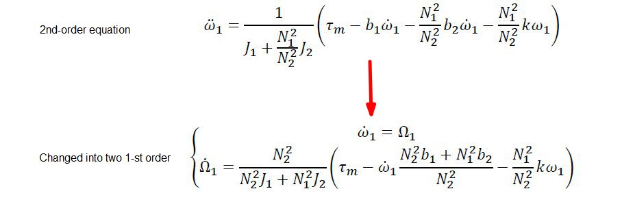
Higher-order ODEs
- Converts higher-order equations to systems of first-order ODEs
- Applies to problems like mechanical vibrations (spring-mass systems) and circuit analysis
- Requires careful handling of initial conditions for all derivatives
- May exhibit increased sensitivity to errors compared to single first-order equations
Limitations and challenges
- Understanding the limitations of Euler's method in Numerical Analysis II highlights the need for more advanced techniques
- Recognizing these challenges motivates the development and study of alternative numerical methods
- Provides context for evaluating the suitability of different numerical approaches for specific problems
Stiffness issues
- Occurs in systems with multiple time scales or large differences in rate constants
- Requires extremely small step sizes for stability, leading to high computational cost
- Euler's method performs poorly on stiff problems, often resulting in numerical instability
- Motivates the use of implicit methods or specialized stiff solvers (Gear's method)
Accuracy vs computational cost
- Improving accuracy by decreasing step size increases the number of computations
- Trade-off between solution accuracy and computational resources (time, memory)
- Global error grows linearly with the number of steps, limiting achievable accuracy
- More sophisticated methods (Runge-Kutta, multistep methods) offer better accuracy-to-cost ratios
Comparison with other methods
- Euler's method serves as a baseline for comparing more advanced numerical techniques
- Generally less accurate than higher-order methods like Runge-Kutta for a given step size
- Simpler to implement and analyze, making it valuable for educational purposes
- May be preferred for certain real-time applications where computational speed is critical
Numerical examples
- Numerical examples in Numerical Analysis II provide concrete illustrations of Euler's method in action
- These examples demonstrate both the capabilities and limitations of the method
- Analyzing specific cases helps develop intuition for the behavior of numerical solutions
Simple harmonic oscillator
- Models a mass on a spring with no damping:
- Converted to a system of first-order ODEs:
- Euler's method typically shows energy drift, failing to preserve the oscillation amplitude
- Illustrates the importance of symplectic integrators for Hamiltonian systems
Population growth models
- Applies to logistic growth equation:
- Demonstrates Euler's method for non-linear ODEs
- Shows how step size affects the accuracy of capturing the S-shaped growth curve
- Highlights potential issues with negative population values for large step sizes
Nonlinear systems
- Applies to systems like the Lorenz equations for atmospheric convection
- Illustrates chaotic behavior and sensitivity to initial conditions
- Demonstrates limitations of Euler's method for long-term predictions in chaotic systems
- Shows how numerical errors can lead to qualitatively different solutions
Software implementation
- Implementing Euler's method in software reinforces programming skills essential in Numerical Analysis II
- Provides hands-on experience with numerical algorithm implementation and testing
- Demonstrates the importance of proper software design in scientific computing
MATLAB code examples
- Utilizes MATLAB's vectorization capabilities for efficient implementation
- Basic Euler method function:
</>MATLABfunction [t, y] = euler(f, tspan, y0, h) t = tspan(1):h:tspan(2); y = zeros(length(t), length(y0)); y(1,:) = y0; for i = 1:length(t)-1 y(i+1,:) = y(i,:) + h * f(t(i), y(i,:))'; end end
- Demonstrates how to handle systems of equations and plot results
- Includes error analysis and comparison with built-in ODE solvers
Python libraries for Euler's method
- Utilizes NumPy for efficient numerical computations
- SciPy's
odeintfunction provides a reference for comparison - Example implementation using Python:
</>Pythonimport numpy as np def euler(f, y0, t): y = np.zeros((len(t), len(y0))) y[0] = y0 for i in range(1, len(t)): y[i] = y[i-1] + (t[i] - t[i-1]) * f(y[i-1], t[i-1]) return y
- Demonstrates integration with matplotlib for visualization of results
Visualization techniques
- Utilizes phase plots for systems of ODEs to show solution trajectories
- Employs error plots to visualize the difference between Euler's method and exact solutions
- Creates animations to illustrate the step-by-step progression of the numerical solution
- Uses logarithmic plots to display error growth and convergence behavior
Advanced topics
- Advanced topics in Euler's method connect to broader themes in Numerical Analysis II
- These concepts bridge the gap between basic numerical methods and more sophisticated techniques
- Understanding these advanced topics provides insight into current research areas in numerical analysis
Adaptive step size control
- Dynamically adjusts step size based on local error estimates
- Improves efficiency by using larger steps where the solution changes slowly
- Implements error control using techniques like step doubling or embedded Runge-Kutta methods
- Balances accuracy requirements with computational cost
Symplectic Euler method
- Designed for Hamiltonian systems to preserve energy and phase space volume
- Splits the system into position and momentum updates
- Provides better long-term stability for oscillatory problems (planetary motion)
- Serves as an introduction to more advanced symplectic integrators
Euler's method for PDEs
- Extends the concept to partial differential equations using finite difference methods
- Applies to problems like the heat equation or wave equation
- Introduces stability considerations specific to PDEs (CFL condition)
- Demonstrates the connection between ODEs and discretized PDEs in numerical analysis