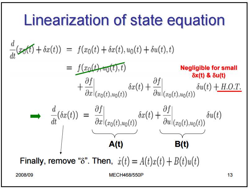
transforms nonlinear systems into equivalent linear ones through coordinate changes and state feedback. This simplifies control design by allowing linear techniques to be applied to nonlinear systems, making complex problems more manageable.
The method works for feedback linearizable systems that meet specific conditions. By converting nonlinear dynamics into linear ones, we can use familiar tools like pole placement and optimal control to achieve desired performance in the original system.
Input-State Linearization Concept
Overview of Input-State Linearization
Top images from around the web for Overview of Input-State Linearization
Control of a SCARA Robot Using Feedback Linearization and Kalman Filter Observer|crimson ... View original
Is this image relevant?
Input-state Linearization of Mechanical System View original
Is this image relevant?
control theory - Derivation for state equation linearization - Mathematics Stack Exchange View original
Is this image relevant?
Control of a SCARA Robot Using Feedback Linearization and Kalman Filter Observer|crimson ... View original
Is this image relevant?
Input-state Linearization of Mechanical System View original
Is this image relevant?
1 of 3
Input-state linearization transforms a nonlinear system into an equivalent linear system through a change of coordinates and state feedback
Simplifies the analysis and design of nonlinear control systems by converting them into linear systems, which have well-established control techniques
Applicable to a class of nonlinear systems called feedback linearizable systems, which satisfy certain conditions on their structure and
Transformed Linear System Properties
The transformed linear system obtained through input-state linearization retains the same state variables as the original nonlinear system
The dynamics of the transformed system are now linear with respect to the new input
Enables the application of linear control techniques, such as pole placement and optimal control, to nonlinear systems (LQR, pole placement)
Conditions for Input-State Linearization
Necessary and Sufficient Conditions
Consider a nonlinear system described by the state equations: x˙=f(x)+g(x)u, where x is the state vector, u is the input, and f(x) and g(x) are smooth vector fields
The vector fields g(x),adfg(x),...,adn−1fg(x) must be linearly independent
adfg(x) denotes the of f(x) and g(x)
n is the dimension of the state space
The distribution spanned by the vector fields g(x),adfg(x),...,adn−2fg(x) must be involutive
The Lie bracket of any two vector fields in the distribution is also in the distribution
Diffeomorphism for Linearization
If the necessary and sufficient conditions are satisfied, there exists a diffeomorphism that transforms the nonlinear system into an equivalent linear system
A diffeomorphism is a smooth and invertible transformation
The diffeomorphism consists of a change of coordinates z=T(x) and a law u=α(x)+β(x)v
v is the new input to the linearized system
The transformed linear system has the form z˙=Az+Bv, where A and B are constant matrices determined by the diffeomorphism
Linearization of Nonlinear Systems
Transformation Process
Given a nonlinear system satisfying the conditions for input-state linearization, find the diffeomorphism that linearizes the system
The change of coordinates z=T(x) is obtained by solving partial differential equations derived from the Lie derivatives of the output function along f(x) and g(x)
The state feedback control law u=α(x)+β(x)v is determined by the choice of the new input v and the requirement to cancel out nonlinearities in the system dynamics
Transformed Linear System
The resulting transformed linear system has the form z˙=Az+Bv, where A and B are constant matrices, and v is the new input
The transformed system preserves the state variables of the original nonlinear system but has linear dynamics with respect to the new input v
Input-state linearization can be applied to various classes of nonlinear systems (feedback linearizable systems, strict feedback systems, pure feedback systems)
State Feedback Control for Linearized Systems
Controller Design
Once a nonlinear system is transformed into an equivalent linear system, linear control techniques can be applied to design state feedback controllers
The state feedback control law for the linearized system has the form v=−Kz, where K is the feedback gain matrix and z is the state vector of the linearized system
The feedback gain matrix K can be designed using pole placement techniques to achieve desired closed-loop pole locations
Desired pole locations are chosen based on performance specifications (settling time, overshoot, margins)
Optimal control techniques, such as linear quadratic regulator (LQR) design, can also be used to determine the feedback gain matrix K that minimizes a quadratic cost function
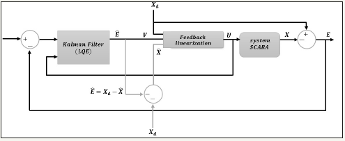
Nonlinear Controller Implementation
The designed state feedback controller for the linearized system is transformed back to the original nonlinear system using the inverse of the diffeomorphism obtained during input-state linearization
The resulting nonlinear state feedback controller achieves the desired closed-loop performance for the original nonlinear system
Robustness and performance trade-offs should be considered when designing state feedback controllers for input-state linearized systems
The linearization is valid only in a neighborhood of the operating point
Key Terms to Review (18)
Aerospace Control: Aerospace control refers to the techniques and strategies employed to manage and regulate the behavior of aerospace systems, including aircraft and spacecraft. It integrates various nonlinear control methods to ensure stability, precision, and adaptability in the highly dynamic and uncertain environments typical of aerospace operations. This field is crucial for enhancing performance, safety, and reliability in both commercial and military aviation as well as space exploration.
Controllability: Controllability refers to the ability of a system to be controlled to any desired state within a finite amount of time using suitable control inputs. It is a crucial property in system theory, indicating whether the system can be manipulated through its inputs to achieve specific performance objectives. Understanding controllability connects to various concepts such as state representation, transformations, and optimization strategies in control design.
Dead Zone: A dead zone refers to a range of input values for which a system does not respond or produces no output, even when the input is applied. This nonlinearity is crucial when analyzing control systems, as it can impact the overall performance and stability of both linear and nonlinear systems. Understanding dead zones helps in designing systems that account for this behavior, particularly in applications requiring precision, such as robotics and automation.
Differential geometric techniques: Differential geometric techniques are mathematical tools that utilize concepts from differential geometry to analyze and design control systems. These techniques often involve the study of manifolds, tangent spaces, and curvature to understand system behavior, particularly for nonlinear systems. By applying these concepts, one can transform complex nonlinear dynamics into more manageable forms, facilitating the design of effective control strategies.
Feedback linearization: Feedback linearization is a control technique that transforms a nonlinear system into an equivalent linear system by applying a feedback law that cancels the nonlinear dynamics. This method allows for the use of linear control techniques to stabilize and control nonlinear systems effectively, making it crucial in various engineering applications.
Hermann W. Kalman: Hermann W. Kalman was a prominent mathematician and engineer known for his groundbreaking work in control theory, particularly the development of the Kalman filter, which revolutionized the fields of control systems and estimation theory. His contributions laid the foundation for modern nonlinear control systems, enhancing the ability to analyze and design systems that can be linearized around operating points.
Input-state linearization: Input-state linearization is a control technique used to transform a nonlinear system into an equivalent linear system through a suitable choice of input and state variables. This method relies on the concept of feedback linearization, where the nonlinear dynamics of the system are canceled out by appropriately designed input signals, resulting in a system that can be analyzed and controlled using linear control methods. It is particularly useful in systems where exact feedback linearization is possible, allowing for easier stability analysis and controller design.
Lie Bracket: The Lie bracket is a mathematical operation that takes two vector fields and produces another vector field, reflecting the non-commutative nature of their flows. It provides a way to capture the infinitesimal behavior of vector fields and is crucial in understanding the structure of nonlinear systems, particularly when performing input-state linearization.
Lie's Theorem: Lie's Theorem states that if a nonlinear system can be transformed into a linear one using state feedback, then the system's dynamics can be analyzed and controlled more easily. This theorem is significant because it provides a method for determining when input-state linearization is possible, thereby allowing control engineers to simplify the analysis of nonlinear systems and design controllers effectively.
Local coordinates: Local coordinates refer to a coordinate system that is defined in a neighborhood around a specific point in a nonlinear system. This concept is particularly important when linearizing a nonlinear system at a given operating point, as it allows for simpler analysis and control design by focusing on the behavior of the system in a localized region.
Model uncertainty: Model uncertainty refers to the lack of perfect knowledge regarding the mathematical representation of a system, which can lead to discrepancies between the actual system behavior and the model predictions. This concept is crucial because it affects the performance and stability of control strategies, making it essential to account for such uncertainties in the design and analysis of nonlinear control systems.
Non-minimum phase behavior: Non-minimum phase behavior refers to a system characteristic where the initial response to a change in input is in the opposite direction of the desired outcome before eventually moving towards it. This type of behavior can complicate control system design and performance, especially in systems that are intended to be controlled using techniques like input-state linearization.
Picard-Lindelöf Theorem: The Picard-Lindelöf Theorem, also known as the Cauchy-Lipschitz theorem, establishes the conditions under which a system of ordinary differential equations has a unique solution. This theorem is crucial in understanding the behavior of dynamical systems and plays a significant role in input-state linearization, where the ability to find unique solutions is fundamental for analyzing the controllability and stability of nonlinear systems.
Robotic manipulation: Robotic manipulation refers to the ability of a robot to interact with and control physical objects in its environment through various actions such as grasping, lifting, and moving. This capability is essential for tasks ranging from simple object handling to complex assembly operations. It combines elements of perception, planning, and control, allowing robots to perform tasks autonomously or collaboratively with humans.
S. sastry: s. sastry refers to the contributions of Shankar Sastry in the field of nonlinear control systems, particularly his work on input-state linearization and parameter estimation. His research emphasizes the importance of understanding how to manipulate nonlinear systems to achieve desired behaviors by transforming them into linear forms and using adaptive methods for system identification.
Saturation: Saturation refers to the condition where a system reaches its maximum capacity, leading to a non-linear response to inputs. This concept is crucial in understanding how systems behave differently under extreme conditions, as it signifies a limit beyond which the output does not continue to increase in proportion to the input. It highlights the fundamental differences between linear and nonlinear systems, where saturation can cause unexpected behaviors such as hysteresis or dead zones, and has significant implications for control strategies and stability in various applications.
Stability: Stability refers to the ability of a system to return to its equilibrium state after a disturbance. In control systems, it is crucial for ensuring that the system behaves predictably and does not diverge uncontrollably from desired performance. Various methods and concepts are used to analyze stability, including feedback mechanisms and control strategies that can shape system dynamics.
State Feedback Control: State feedback control is a control strategy that uses the current state of a system to compute control inputs aimed at achieving desired behavior. By utilizing state variables, this approach can effectively stabilize and regulate system performance, making it especially useful for nonlinear systems. This technique helps in designing controllers that can adaptively respond to changing conditions and ensures robust performance across different operating points.