AP exam review verified for 2027

AP Physics 2 Unit 10 Review: Electric Force, Field, and Potential

Review AP Physics 2 Unit 10 to build a complete picture of electrostatics, from Coulomb's law and charge conservation through electric fields, potential energy, voltage, and capacitors. This unit carries 15-18% of the exam and connects directly to circuits in Unit 11.

Use the topic guides, key terms, and available practice questions to work through every concept from electric force to conservation of electric energy.

What is AP Physics 2 unit 10?

Unit 10 is the foundation of all electricity content in AP Physics 2. It introduces the electric force as a field force that obeys Newton's laws, then builds upward through field maps, potential energy, voltage, and energy storage in capacitors.

Unit 10 covers electric charge and Coulomb's law, conservation and transfer of charge, electric fields and field maps, electric potential energy, electric potential and equipotential lines, parallel-plate capacitors, and conservation of electric energy for moving charges.

Forces and Fields

Coulomb's law gives the magnitude of the electrostatic force between two point charges: |F| = k|q1 q2|/r^2. The electric field E = F/q describes the force per unit charge at any point in space, and the net field from multiple charges is found by vector superposition.

Potential Energy and Voltage

Electric potential energy for a pair of point charges is U_E = kq1q2/r. Electric potential V = U_E/q is a scalar, so contributions from multiple charges add directly. Potential difference delta V = delta U_E / q connects energy changes to voltage, and equipotential lines are always perpendicular to field vectors.

Capacitors and Energy Conservation

A parallel-plate capacitor stores charge according to C = Q/delta V, with capacitance set by C = kappa epsilon_0 A/d. Stored energy is U_C = (1/2)Q delta V. When a charge moves through a potential difference, delta U_E = q delta V, and conservation of energy links that change to a change in kinetic energy.

Everything connects through energy

The deepest thread in Unit 10 is that electric force is conservative, meaning you can track every interaction through potential energy and voltage instead of force vectors alone. Coulomb's law, field maps, equipotential lines, capacitor storage, and particle acceleration are all different windows into the same energy bookkeeping. Understanding that connection prepares you for circuits in Unit 11, where voltage and energy transfer drive every calculation.

AP Physics 2 unit 10 topics

10.1

Electric Charge and Electric Force

Introduces charge as a fundamental property, the elementary charge e, the point charge model, Coulomb's law |F| = k|q1 q2|/r^2, electric permittivity, and the comparison of electric and gravitational forces.

open guide
10.2

Conservation of Electric Charge and the Process of Charging

Covers conservation of charge, charging by friction, contact, and induction, induced charge separation in neutral objects, and grounding.

open guide
10.3

Electric Fields

Defines the electric field E = F/q, covers vector superposition of fields from multiple charges, field line maps, and the distinct field behavior inside conductors versus insulators in electrostatic equilibrium.

open guide
10.4

Electric Potential Energy

Defines U_E = kq1q2/r for a pair of point charges, explains the sign convention, and extends to multi-charge systems using pairwise summation.

open guide
10.5

Electric Potential

Introduces electric potential V = kq/r as a scalar, scalar superposition, potential difference delta V = delta U_E / q, equipotential lines, and the relationship |E| = |delta V / delta r|.

open guide
10.6

Capacitors

Covers parallel-plate capacitor geometry, C = Q/delta V, C = kappa epsilon_0 A/d, the effect of dielectrics, the uniform field between plates, and stored energy U_C = (1/2) Q delta V.

open guide
10.7

Conservation of Electric Energy

Applies conservation of energy to charged particles moving through potential differences using delta U_E = q delta V and delta K = -delta U_E, with attention to sign conventions for positive and negative charges.

open guide
practice snapshot

Hardest AP Physics 2 unit 10 topics

This snapshot uses Fiveable practice activity to show where students tend to miss questions and which review moves are worth prioritizing first.

59%average MCQ accuracy

Across 1.9k multiple-choice practice attempts for this unit.

1.9kMCQ attempts

Practice activity included in this snapshot.

16%average FRQ score

Across 5 scored free-response attempts for this unit.

Hardest topics in unit 10

MCQ miss rate
10.7

Review Conservation of Electric Energy with attention to how the concept appears in AP-style source and evidence questions.

52%109 tries
10.1

Review Electric Charge and Electric Force with attention to how the concept appears in AP-style source and evidence questions.

45%530 tries
10.2

Review Conservation of Electric Charge and the Process of Charging with attention to how the concept appears in AP-style source and evidence questions.

26%284 tries

Unit 10 review notes

10.1

Electric Charge and Coulomb's Law

Charge is a fundamental property of matter, quantized in units of the elementary charge e = 1.602 x 10^-19 C. Protons carry +e, electrons carry -e, and neutrons carry no charge. Coulomb's law gives the magnitude of the electrostatic force between two point charges: |F_E| = k|q1 q2|/r^2, where k = 8.99 x 10^9 N m^2/C^2. The force is attractive for opposite signs and repulsive for like signs, and it falls off as 1/r^2. Electric permittivity epsilon_0 appears in the equivalent form |F_E| = |q1 q2| / (4 pi epsilon_0 r^2). For any object with both mass and charge, the gravitational force is almost always negligible compared to the electrostatic force at small scales; gravity dominates at large scales only because macroscopic objects are nearly electrically neutral.

  • Elementary charge: e = 1.602 x 10^-19 C; the smallest indivisible unit of charge, carried by a proton (+e) or electron (-e).
  • Point charge model: Treats a charged object as if all its charge is concentrated at a single point, valid when the object's size is negligible compared to the distances involved.
  • Coulomb's law: |F_E| = k|q1 q2|/r^2; force is proportional to each charge and inversely proportional to the square of the separation distance.
  • Electric permittivity: epsilon_0 = 8.85 x 10^-12 F/m; measures how easily a medium is polarized; appears in the denominator of Coulomb's law as 4 pi epsilon_0.
  • Electric vs. gravitational force: Both follow inverse-square laws, but electrostatic forces can be attractive or repulsive while gravity is always attractive; electrostatic forces handle at atomic and molecular scales.
If the distance between two charges doubles, by what factor does the electrostatic force change? (Answer: it decreases by a factor of 4, since force is proportional to 1/r^2.)
PropertyGravitational ForceElectrostatic Force
SourceMassElectric charge
DirectionAlways attractiveAttractive or repulsive
LawF = Gm1m2/r^2F = k|q1 q2|/r^2
Dominates atLarge (astronomical) scalesSmall (atomic/molecular) scales
10.2

Conservation of Charge and Charging Methods

The net charge of an isolated system never changes; any change in a system's charge requires a transfer of charge to or from its surroundings. Charging by friction transfers electrons between materials based on their positions in the triboelectric series. Charging by contact (conduction) transfers electrons when objects touch. Charging by induction redistributes charge within a neutral object without direct contact, and grounding allows excess charge to flow to or from Earth, leaving the object with a net charge. Induced charge separation can occur in neutral objects and does not change their net charge.

  • Conservation of charge: The total charge of an isolated system is constant; charge is neither created nor destroyed, only transferred.
  • Charging by friction: Electrons transfer between two materials rubbed together; the material that gains electrons becomes negative, the one that loses electrons becomes positive.
  • Charging by induction: A nearby charged object redistributes charges in a neutral conductor without touching it; grounding during induction leaves the conductor with a net charge opposite to the inducing charge.
  • Induced charge separation: The electrostatic force from an external charge rearranges charges within a neutral object, creating a polarized distribution without changing the net charge.
  • Grounding: Connecting a charged object to Earth allows charge to flow until the object reaches electrical neutrality or a defined charge state.
A neutral metal sphere is brought near a positively charged rod without touching. The near side of the sphere becomes negative. If the sphere is then grounded while the rod is still nearby, what is the sphere's net charge after the ground connection is removed and the rod is taken away? (Answer: the sphere is left with a net negative charge.)
10.3

Electric Fields

The electric field at a point is defined as E = F_E / q, where q is a small positive test charge that does not disturb the field. Fields point away from positive source charges and toward negative source charges. For a single point charge, E = kq/r^2. The net field from multiple charges is the vector sum of individual fields (superposition). In electrostatic equilibrium, the field inside a solid conductor is zero and the field at the surface is perpendicular to the surface; all excess charge resides on the surface. Inside an insulator, the field can be nonzero. Electric field line maps show direction and relative magnitude: denser lines indicate stronger fields.

  • Electric field definition: E = F_E / q; the force per unit positive test charge at a point in space; units are N/C.
  • Superposition principle: The net electric field at any point is the vector sum of the fields produced by each individual charge.
  • Field inside a conductor: Zero in electrostatic equilibrium; any excess charge distributes on the outer surface, and the field at the surface is perpendicular to it.
  • Field inside an insulator: Can be nonzero because charge is distributed throughout the volume, not just on the surface.
  • Electric field lines: Visual representation of the field; direction shows force on a positive test charge, and line density indicates field magnitude.
Two equal positive charges are placed 0.2 m apart. Where along the line connecting them is the net electric field zero? (Answer: at the midpoint, by symmetry, since the two equal fields point in opposite directions and cancel.)
10.4

Electric Potential Energy

The electric potential energy of a two-charge system equals the work an external agent must do to bring the charges from infinitely far apart to their current separation: U_E = kq1q2/r. The sign of U_E depends on the product q1q2: positive for like charges (energy stored in repulsion) and negative for opposite charges (energy released in attraction). For a system of more than two charges, sum the potential energy of every unique pair: U_total = sum of k qi qj / r_ij for all i < j. The reference point is U_E = 0 at infinite separation.

  • Electric potential energy formula: U_E = kq1q2/r; positive when charges have the same sign, negative when they have opposite signs.
  • Work to assemble charges: U_E equals the work done by an external force to bring charges from infinity to their current positions against (or with) the electric force.
  • Pairwise superposition: For a system of N charges, total U_E is the sum of kqiqj/rij for every unique pair; each pair is counted once.
  • Sign convention: Negative U_E means the configuration is energetically favorable (charges attracted); positive U_E means work was done against repulsion.
Three charges +q, +q, and -q are placed at the corners of an equilateral triangle with side length d. What is the sign of the total electric potential energy of the system? (Hint: identify the three pairs and their signs, then sum.)
10.5

Electric Potential and Equipotential Lines

Electric potential V is the electric potential energy per unit charge at a point: V = U_E / q. For a point charge, V = kq/r. Because potential is a scalar, contributions from multiple charges add algebraically: V = k sum(qi/ri). Potential difference delta V = delta U_E / q tells how much energy per coulomb changes when a charge moves between two points. The average electric field magnitude between two points is |E| = |delta V / delta r|, so field vectors point from high to low potential. Equipotential lines (isolines) connect points of equal V and are always perpendicular to field vectors. No work is done moving a charge along an equipotential. Conductors in electrostatic equilibrium are equipotential surfaces.

  • Electric potential: V = U_E / q; scalar quantity in volts (V = J/C); for a point charge, V = kq/r.
  • Scalar superposition: Total potential from multiple charges is V = k sum(qi/ri); add algebraically, not as vectors.
  • Potential difference: delta V = delta U_E / q; the change in potential energy per coulomb when a charge moves between two points.
  • Equipotential lines: Lines of equal electric potential; always perpendicular to electric field vectors; no work is done moving a charge along them.
  • Field-potential relationship: |E| = |delta V / delta r|; the electric field points in the direction of decreasing potential.
A positive charge moves from a region of high potential to low potential. Does its electric potential energy increase or decrease? Does it speed up or slow down? (Answer: U_E decreases; kinetic energy increases; the charge speeds up.)
FeatureElectric FieldElectric Potential
TypeVectorScalar
Formula (point charge)E = kq/r^2V = kq/r
SuperpositionVector sumAlgebraic sum
RelationshipPoints from high to low VDecreases in direction of E
EquipotentialsPerpendicular to field linesLines/surfaces of constant V
10.6

Capacitors

A parallel-plate capacitor consists of two conducting plates that store equal and opposite charge Q separated by a gap d. Capacitance is defined as C = Q / delta V and depends only on geometry and material: C = kappa epsilon_0 A / d, where kappa is the dielectric constant of the material between the plates, A is the plate area, and d is the separation. The uniform electric field between the plates is E = Q / (kappa epsilon_0 A). Inserting a dielectric increases capacitance by reducing the effective field through induced polarization. Energy stored in a capacitor is U_C = (1/2) Q delta V = (1/2) C (delta V)^2 = Q^2 / (2C).

  • Capacitance definition: C = Q / delta V; the ratio of stored charge to the potential difference across the plates; units are farads (F).
  • Parallel-plate capacitance: C = kappa epsilon_0 A / d; increases with larger plate area, decreases with larger gap, increases with higher dielectric constant.
  • Dielectric constant kappa: A dimensionless factor greater than 1 that multiplies epsilon_0 when a material fills the gap; increases capacitance by reducing the electric field for a given charge.
  • Stored energy: U_C = (1/2) Q delta V = (1/2) C (delta V)^2 = Q^2 / (2C); energy is stored in the electric field between the plates.
  • Uniform field between plates: E = Q / (kappa epsilon_0 A); constant in magnitude and direction between ideal parallel plates, enabling projectile-like analysis of charged particles.
A capacitor is charged to voltage delta V and then disconnected from the battery. If the plate separation is doubled, what happens to the capacitance, the voltage, and the stored energy? (Answer: C halves, delta V doubles since Q is fixed, and U_C doubles.)
10.7

Conservation of Electric Energy

When a charged object moves between two points with different electric potentials, its electric potential energy changes by delta U_E = q delta V. Because the electrostatic force is conservative, energy is conserved: any decrease in U_E appears as an increase in kinetic energy, and vice versa. For a charge moving freely in an electric field, delta K = -delta U_E. This is the electric analog of conservation of mechanical energy. Sign conventions matter: a positive charge moving from high to low potential loses potential energy and gains kinetic energy; a negative charge moving from high to low potential gains potential energy and loses kinetic energy.

  • Energy change formula: delta U_E = q delta V; the change in electric potential energy equals the charge times the potential difference.
  • Conservation of energy: delta K + delta U_E = 0 for a charge moving freely in an electric field; kinetic and potential energy trade off.
  • Sign convention for charges: Positive charges accelerate from high to low potential (losing U_E, gaining K); negative charges accelerate from low to high potential.
  • Work done by electric field: W = -delta U_E = q delta V; positive work by the field increases kinetic energy.
An electron (charge -e) moves from a point at V = 0 V to a point at V = +100 V. Does it speed up or slow down? (Answer: delta U_E = (-e)(+100) < 0, so U_E decreases and K increases; the electron speeds up.)

Practice AP Physics 2 unit 10 questions

Try AP-style multiple-choice questions and written prompts after you review the notes.

Example stimulus-based MCQs

open all practice
Topic 10.1

Electric Charge and Electric Force practice question

diagram

A uniformly charged solid insulating cylinder and a solid conducting cylinder of the same radius R and length carry equal total positive charges. The figure shows cross-sectional views of both cylinders with representative electric field vectors drawn at several interior points.

Question

A student claims the electric field vectors inside the insulating cylinder are valid, but any nonzero field inside the conducting cylinder is not. Which evaluation is best?

Correct, because insulators can have nonzero internal fields, while conductors in equilibrium cannot.

Incorrect, because both conductors and insulators must have zero field inside when charged equally.

Correct, because surface charge in the insulator creates the internal field, unlike the conductor.

Incorrect, because the insulating cylinder must also have zero field by symmetry.

Topic 10.2

Conservation of Electric Charge and the Process of Charging practice question

diagram

Two identical neutral metal spheres, P and Q, rest on insulating stands and are in contact. A negatively charged rod is brought near sphere P, as shown. While the rod remains in place, the spheres are separated. The rod is then removed.

Question

Which of the following correctly compares the final net charges on sphere P (Q_P) and sphere Q (Q_Q) after the rod is removed?

Q_P is positive and Q_Q is negative, with |Q_P| = |Q_Q|.

Q_P is negative and Q_Q is positive, with |Q_P| = |Q_Q|.

Q_P is negative and Q_Q is positive, with |Q_P| > |Q_Q|.

Q_P is neutral and Q_Q is neutral, because the rod never touched either sphere.

Example FRQs

open all FRQs
FRQ

Parallel plate capacitor with charged particle motion

2. Two large, parallel conducting plates of area A=0.040 m2A = 0.040\ \text{m}^2 are separated by a distance d=6.0×10³ md = 6.0× 10^{-3}\ \text{m}, as shown in Figure 1. The plates are initially uncharged and are connected to a battery that maintains a potential difference of ΔV=480 V\Delta V = 480\ \text{V} with the top plate at higher potential. The region between the plates is initially air, which can be treated as vacuum with permittivity ε0=8.85×10¹² F/m\varepsilon_0 = 8.85× 10^{-12}\ \text{F/m}. A small insulating sphere of mass m=2.0×10⁴ kgm = 2.0× 10^{-4}\ \text{kg} carrying charge q=+3.0×10⁹ Cq = +3.0× 10^{-9}\ \text{C} is released from rest midway between the plates. Take g=9.8 m/s2g = 9.8\ \text{m/s}^2.

Figure 1. Parallel-plate capacitor connected to a 480 V battery with a positively charged insulating sphere released midway between the plates.

Create a clean, black-and-white physics apparatus diagram on a plain white background.

Overall layout (must be unambiguous):
- The diagram is in landscape orientation.
- Two large, perfectly horizontal, perfectly parallel conducting plates are drawn as long, thin rectangles spanning nearly the full width of the diagram.
- The top plate sits in the upper quarter of the diagram; the bottom plate sits in the lower quarter, directly below it.
- The empty gap (air/vacuum region) between plates is clearly visible and uniform.

Plates (geometry and labels):
- Top plate: a long horizontal rectangle. Place a bold plus sign “+” centered on the top plate to indicate it is at higher potential.
- Bottom plate: a matching long horizontal rectangle directly below. Place a bold minus sign “−” centered on the bottom plate to indicate it is at lower potential.
- To the right side of the plates, draw a vertical double-headed dimension arrow spanning exactly from the inner face of the top plate to the inner face of the bottom plate.
- Next to that dimension arrow, place the text label “d = 6.0×10⁻³ m”. The arrowheads must touch the two inner plate surfaces to show the separation precisely.
- Near the plates (but not on the dimension arrow), include the plate area label as plain text: “A = 0.040 m²”. This label must be clearly associated with the plates (placed between the plates near one side, or just above the top plate near one end).

Battery and connections (must show closed circuit):
- Draw a battery symbol to the right of the plates, vertically oriented (one long line and one short line).
- Connect the top plate to the positive terminal (long line) of the battery with a solid wire, and connect the bottom plate to the negative terminal (short line) with a solid wire.
- Place the text “ΔV = 480 V” immediately adjacent to the battery symbol.
- The wires must clearly attach to the plates at their right ends, forming an unmistakable connection.

Charged sphere (position and labels):
- Between the plates, draw a small solid circle representing a small insulating sphere.
- Place the sphere exactly halfway between the plates vertically (center of the gap), and also centered left-to-right between the plate ends (sphere centered in the middle of the capacitor region).
- Place the label “+q” immediately next to the sphere, and also include the explicit numeric charge as a second line of text near the sphere: “q = +3.0×10⁻⁹ C”.
- Include the mass near the sphere as text: “m = 2.0×10⁻⁴ kg”.

Vertical position axis (y-direction definition):
- On the left side of the plates, draw a vertical axis arrow pointing upward.
- Label the axis “y” next to the arrow.
- Mark the bottom plate level as “y = 0” with a small tick and label aligned with the bottom plate.
- Mark the top plate level as “y = d” with a small tick and label aligned with the top plate.

Styling constraints:
- Use consistent line thickness: plates slightly thicker than wires; dimension arrows and axis arrows medium thickness.
- No perspective drawing: all lines must be strictly horizontal or vertical.
- No additional text beyond the specified labels (+, −, A, d, ΔV, y, y = 0, y = d, q value, m value).

Figure dot. Force diagram. Dot represents the center of mass of the charged insulating sphere just after release.

Create a minimal free-body diagram region on a plain white background.

Object (required):
- Draw a single small filled dot centered in the diagram.
- Place the label “sphere” or “charged sphere” directly below the dot in small text.

Forces (student-drawn space must be clear, but force directions must be implied by context of the problem):
- Do NOT pre-draw any force arrows; leave the area around the dot empty so students can add arrows.
- Ensure there is ample blank space above and below the dot for two opposite vertical arrows.

Context cues (non-numeric, allowed):
- Add a faint note near the top margin: “Draw and label all forces on the sphere.”
- Do not include any coordinate axes, any plate drawings, or any numeric values in this force-diagram figure.

Styling:
- The dot is the only shape; all else is blank whitespace with the single instruction text and the object label.
A.

On the dot shown in Figure dot, representing the charged sphere just after it is released, draw and label the forces that are exerted on the sphere. Each force must be represented by a distinct arrow starting on, and pointing away from, the dot.

B.

Derive an expression for the magnitude of the electric field EE between the plates in terms of ΔV\Delta V and dd. Begin your derivation by writing a fundamental physics principle or an equation from the reference information. Then use your result to derive an expression for the magnitude of the net force on the sphere in terms of qq, ΔV\Delta V, dd, mm, and gg.

Figure 2. Axes for electric potential V as a function of vertical position y between the plates (y=0 at bottom plate, y=d at top plate).

Create a blank set of graph axes (no curve pre-drawn) on a plain white background.

Axes (all numeric scales must be shown):
- Horizontal axis: label centered below the axis as “y (m)”.
- Horizontal axis range: start at 0 on the far left and end at 6.0×10⁻³ on the far right.
- Horizontal tick marks: show exactly four equal intervals between 0 and 6.0×10⁻³, so there are five labeled ticks total.
- Horizontal tick labels (left to right): “0”, “1.5×10⁻³”, “3.0×10⁻³”, “4.5×10⁻³”, “6.0×10⁻³”.
- Vertical axis: label along the left side as “V (V)”.
- Vertical axis range: start at 0 at the bottom and end at 480 at the top.
- Vertical tick marks: label ticks every 120 V so there are five labeled ticks total.
- Vertical tick labels (bottom to top): “0”, “120”, “240”, “360”, “480”.
- The origin is the bottom-left intersection and must be labeled “0” on both axes at the intersection (single shared “0” label is acceptable if clearly at the origin).
- Add arrowheads on the positive (right) end of the horizontal axis and the positive (top) end of the vertical axis.

Required marked values for Part C:
- On the left end of the x-axis (at y=0), place a small text annotation just above the axis: “V(0) = 0 V”.
- On the right end of the x-axis (at y=d), place a small text annotation near the right boundary: “V(d) = 480 V”.

No curve yet (this figure is for students to sketch):
- Do not draw the potential curve.
- Do not draw any electric-field arrow on the graph; leave the interior blank so students can add it.

Styling constraints:
- No gridlines.
- Medium-weight black axes, lighter tick marks.
- No title beyond the caption (caption not drawn inside the axes).
C.

On the axes provided in Figure 2, sketch the electric potential V(y)V(y) between the plates as a function of vertical position yy, where y=0y = 0 at the bottom plate and y=dy = d at the top plate. Clearly indicate on your sketch the values V(0)V(0) and V(d)V(d), and draw an arrow on your sketch to indicate the direction of the electric field.

D.

Indicate whether each of the following quantities increases, decreases, or remains the same when the dielectric is inserted while the battery stays connected. A dielectric slab of thickness t=6.0×10³ mt = 6.0× 10^{-3}\ \text{m} (equal to the plate separation) and relative permittivity κ=4.0\kappa = 4.0 is inserted to completely fill the region between the plates while the battery remains connected and maintains ΔV=480 V\Delta V = 480\ \text{V}. The sphere is again placed midway between the plates and released from rest.

Given values: A=0.040 m2A = 0.040\ \text{m}^2, d=6.0×10³ md = 6.0× 10^{-3}\ \text{m}, ΔV=480 V\Delta V = 480\ \text{V}, ε0=8.85×10¹² F/m\varepsilon_0 = 8.85× 10^{-12}\ \text{F/m}, κ=4.0\kappa = 4.0, m=2.0×10⁴ kgm = 2.0× 10^{-4}\ \text{kg}, q=+3.0×10⁹ Cq = +3.0× 10^{-9}\ \text{C}, g=9.8 m/s2g = 9.8\ \text{m/s}^2.

  1. The magnitude of the electric field between the plates
    Increases
    Decreases
    Remains the same
  1. The magnitude of the charge on the top plate
    Increases
    Decreases
    Remains the same
  1. The energy stored in the capacitor
    Increases
    Decreases
    Remains the same

Briefly justify each answer. Your justification must reference conservation of charge and/or the relationship between ΔV\Delta V, EE, capacitance, and energy. Then calculate the new energy stored in the capacitor after the dielectric is inserted.

FRQ

Dielectric permittivity determination in parallel-plate capacitors

3. In Experiment 1, a student is given a parallel-plate capacitor with square conducting plates. The plates can be separated by an adjustable distance d. The region between the plates can be either air or completely filled with a slab of dielectric material. The student is asked to determine the permittivity of the dielectric material and relate the results to electric field and electric potential in the capacitor.

A.

Describe a procedure for collecting data that would allow the student to determine the permittivity ε\varepsilon of the dielectric material. In your description, include the measurements to be made. Include any steps necessary to reduce experimental uncertainty.

B.

Describe how the collected data could be analyzed to determine ε\varepsilon. Include references to appropriate equations and to relationships between measured and known quantities.

Figure 1. Parallel-plate capacitor circuit for measuring charge q and potential difference ΔV with adjustable plate separation d and optional dielectric slab filling the gap.

Black-and-white physics apparatus diagram with all components labeled using printed text. The drawing is arranged left-to-right as a single circuit path across the top half of the page, with instruments branching where stated.

Overall layout and wiring (left to right):
- At the far left is a rectangular DC power supply box labeled exactly: "DC power supply". On its front face are two output terminals: a red (+) terminal on the upper right of the box labeled "+" and a black (−) terminal on the lower right of the box labeled "−".
- A solid wire leaves the + terminal and goes rightward to a single-pole switch symbol located in the left-center of the page. The switch is drawn as an open switch (gap visible) and labeled "Switch" directly above it.
- From the right side of the switch, a solid wire continues rightward to the top plate of the capacitor.
- A second solid wire leaves the − terminal of the DC power supply and runs rightward along the lower part of the circuit to connect to the bottom plate of the capacitor.

Capacitor geometry (center-right of page):
- The parallel-plate capacitor is the dominant central object. It is drawn as two large square plates facing each other with a clear gap between them.
- The plates are oriented vertically (their faces are vertical planes) so the gap between them is horizontal.
- The left plate is connected to the wire coming from the switch; the right plate is connected to the return wire going back to the power supply negative terminal.
- Each plate is explicitly labeled: the left plate label reads "Plate A" and the right plate label reads "Plate B".

Adjustable separation distance d (explicit measurement annotation):
- Between the two plates, draw a double-headed horizontal arrow spanning only the empty gap from the inner face of Plate A to the inner face of Plate B.
- Centered above this double-headed arrow, print the label exactly: "d".
- The arrowheads must touch the inner faces of the two plates to indicate the separation is measured face-to-face.

Ruler for measuring d (explicit placement):
- Directly below the gap (still between the plates), draw a straight ruler aligned horizontally, parallel to the double-headed arrow.
- The ruler’s left end is vertically aligned with the inner face of Plate A, and the ruler’s right end is vertically aligned with the inner face of Plate B, so it visually spans the same separation distance.
- The ruler is labeled "ruler" below it.
- The ruler shows evenly spaced tick marks with longer tick marks every 1 cm and shorter tick marks every 0.5 cm. The visible printed numbers on the ruler are: "0" at the left end, then "1", "2", "3", "4", "5" increasing to the right.

Voltmeter connection (across the plates):
- Above the capacitor, draw a circular voltmeter symbol labeled with a large "V" inside the circle.
- The voltmeter has two leads: one lead connects to the node at Plate A (same node as the wire from the switch), and the other lead connects to the node at Plate B (same node as the return wire).
- Next to the voltmeter circle, print the label exactly: "Voltmeter (measures ΔV)".

Electrometer for charge measurement (series with one plate measurement lead):
- To the right of the capacitor, draw a rectangular instrument box labeled "Electrometer".
- A single wire runs from Plate B to the electrometer input, indicating the electrometer is used to measure the charge on that plate.
- Near the Plate B connection, place the text label exactly: "q (charge on one plate)" with a leader line pointing to Plate B.

Dielectric slab (removable, fully fills the gap when inserted):
- Draw a rectangular slab (same height as the plates) positioned just below and slightly in front of the gap region, with its long dimension vertical to match plate height.
- The slab is labeled "Dielectric slab".
- Show an insertion direction by a single rightward arrow from the slab toward the gap, indicating it slides into the space between the plates.
- Also include a small note printed near the gap: "When inserted, slab completely fills the space between plates".

Clarity requirements:
- All component labels must be placed so no label overlaps any wire or symbol.
- All wires are solid lines with right-angle corners (no diagonal wires), making each electrical connection unambiguous.
- No numerical values are printed on the circuit elements other than the ruler markings described above.

Figure 2. Blank graphing grid for a straight-line plot used to determine capacitance C from measurements of charge q and potential difference ΔV.

A full-page blank Cartesian grid intended for student plotting, with axes, tick marks, numbers, and units areas explicitly defined, but with no data points pre-plotted.

Grid and border:
- A rectangular plotting region occupies most of the figure, with a thin black border.
- Inside the border is a uniform square grid (light lines) with darker grid lines every fifth square to help counting.

Axes (bold, with arrows):
- A bold horizontal axis runs along the bottom of the plotting region with a right-pointing arrowhead at the far right end.
- A bold vertical axis runs along the left side of the plotting region with an upward-pointing arrowhead at the top end.
- The axes intersect at the bottom-left corner of the plotting region, and the origin is labeled with the printed number "0" at that corner.

Numeric scales (must be printed exactly as stated):
- Horizontal axis is intended for potential difference. Print the axis label centered below the axis as: "ΔV (V)".
- Along the horizontal axis, print tick labels at equal spacing: "0", "50", "100", "150", "200", "250". Each labeled tick is marked with a short vertical tick mark.
- The grid must extend one additional unlabeled tick interval beyond 250 to the right so the plotted range clearly includes 0 to 250 with margin.

- Vertical axis is intended for charge in the scaled units used in Table 1. Print the vertical axis label rotated along the left side as: "q (×10⁻⁸ C)".
- Along the vertical axis, print tick labels at equal spacing: "0.0", "0.5", "1.0", "1.5", "2.0", "2.5". Each labeled tick is marked with a short horizontal tick mark.
- The grid must extend one additional unlabeled tick interval above 2.5 so the plotted range clearly includes 0.0 to 2.5 with margin.

Blank plotting area:
- No points, no best-fit line, and no annotations are drawn inside the grid other than the grid lines.
- There is no title inside the plotting area.

Axis labeling spaces:
- Leave clear whitespace just outside the plotting region: below the x-axis label area and to the left of the y-axis label area, so student-added markings do not collide with printed labels.

Consistency with Table 1:
- The chosen printed scales exactly accommodate all Table 1 values: ΔV from 50 to 250 and q from 0.46 to 2.27 in units of ×10⁻⁸ C.

DeltaV (V)

q (x10^-8 C)

50.0

0.46

100.0

0.91

150.0

1.36

200.0

1.82

250.0

2.27

C.

In Experiment 2, the student sets the plate separation to d=3.00×10³ md = 3.00× 10^{-3}\ \text{m} and fully inserts the dielectric so it completely fills the gap between the plates. For each trial, the student charges the capacitor to an absolute potential difference ΔV\Delta V, then disconnects the power supply and uses the electrometer to measure the charge qq on one plate. Table 1 contains the data collected.

i.

Indicate two quantities, either measured quantities from Table 1 or additional calculated quantities, that could be graphed to produce a straight line that could be used to determine the capacitance CC of the capacitor.

Vertical axis: Horizontal axis:

ii.

On Figure 2, create a graph of the quantities indicated in part C(i) that can be used to determine CC.

Use Table 2 to record the data points or calculated quantities that you will plot.

Clearly label the axes, including units as appropriate.

Plot the points you recorded in Table 2.

iii.

Draw a best-fit line for the data graphed in part C(ii).

D.

Using the best-fit line that you drew in part C(iii), calculate an experimental value for the capacitance CC. Using the best-fit line from part C(iii), the student determines that the slope of the graph is 9.10×10¹¹ C/V9.10× 10^{-11}\ \text{C/V}.

FRQ

Charge redistribution and electrostatic forces

1. Two small conducting spheres, Sphere A and Sphere B, are mounted on insulating stands and can be treated as point charges, as shown in Figure 1. Sphere A has mass mA=4.0×10³ kgm_A = 4.0× 10^{-3}\ \text{kg} and initial charge qA,i=+6.0 nCq_{A,i} = +6.0\ \text{nC}. Sphere B has mass mB=4.0×10³ kgm_B = 4.0× 10^{-3}\ \text{kg} and initial charge qB,i=2.0 nCq_{B,i} = -2.0\ \text{nC}. The centers of the spheres are separated by a distance r=0.40 mr = 0.40\ \text{m} in air, which may be treated as vacuum with permittivity ε0=8.85×10¹² F/m\varepsilon_0 = 8.85× 10^{-12}\ \text{F/m}. The spheres are then touched together and separated again so that the final charges on the two identical conducting spheres are equal. Ignore air breakdown and assume the spheres are small compared with rr.

Figure 1. Two identical small conducting spheres on insulating stands separated by r = 0.40 m along the +x direction.

Clean black-line physics setup diagram on a plain white background.

Overall layout:
- A single straight horizontal reference line (thin black) runs across the middle of the figure to represent the line joining the sphere centers (this is the x-axis line of action).
- Sphere A is positioned in the left third of the diagram; Sphere B is positioned in the right third of the diagram.
- The spheres are drawn as identical small circles (same diameter), each with a clearly marked center point (a small filled dot) to emphasize that the center-to-center distance is measured between centers.

Insulating stands:
- Directly beneath each sphere is an insulating stand: a vertical support (thin black line) rising from a small rectangular base.
- Each stand is explicitly labeled with the text “insulating stand” next to it, with a short leader line pointing to the stand.

Labels on spheres (visible text next to each sphere):
- Next to the left sphere, place the label “Sphere A” and directly below it the charge label “q_A,i = +6.0 nC”.
- Next to the right sphere, place the label “Sphere B” and directly below it the charge label “q_B,i = −2.0 nC”.
- The plus and minus signs must be large and unambiguous: “+6.0 nC” has an explicit plus sign; “−2.0 nC” has a clear minus sign.

Separation distance annotation:
- Draw a double-headed horizontal dimension arrow exactly along the center-to-center line connecting the center dot of Sphere A to the center dot of Sphere B.
- Centered above this dimension arrow, place the text label “r = 0.40 m”.
- The arrowheads touch the vertical projection from each sphere’s center (i.e., the dimension is unambiguously center-to-center).

Coordinate axis:
- Near the lower middle portion of the diagram (below the sphere-center line so it does not overlap the distance label), draw a single horizontal axis arrow pointing to the right.
- Label it with “+x” placed just to the right of the arrowhead.
- The +x arrow must be colinear with the line connecting the sphere centers.

No extra quantities:
- Do not show any forces, fields, or additional points in this figure.
- No gridlines and no numerical axes ticks; only the +x direction arrow and the r dimension annotation are present.

Figure 2. Force-direction vectors at Sphere A due to Sphere B (electric and gravitational).

Minimal vector-direction diagram focused on Sphere A, drawn on a plain white background.

Reference objects and axis:
- Show a single point representing the center of “Sphere A” located in the left half of the figure. Mark it with a small filled dot.
- Immediately next to the dot, place the text label “Sphere A”.
- Through the dot, draw a horizontal axis line with a right-pointing arrowhead. Label the arrowhead “+x”. The +x arrow must be perfectly horizontal.

Direction reference to Sphere B:
- To the right of Sphere A (on the same horizontal line), draw a small text-only marker “Sphere B (to the right)” with a short faint guideline arrow pointing rightward. This is only a positional cue; Sphere B itself is not drawn as a full sphere.

Two blank force vectors (student-response arrows):
- From the Sphere A dot, draw two separate blank arrows (no arrow direction chosen by the diagram; both are drawn as empty-outline arrows intended for students to modify/choose direction).
- The first arrow is labeled “Electric force on A due to B, F_E” placed just above the arrow shaft.
- The second arrow is labeled “Gravitational force on A due to B, F_g” placed just below the arrow shaft.

Exact placement and separation of the two arrows:
- Both arrows must start exactly at the Sphere A center dot (same tail point).
- The two arrows are drawn horizontally (colinear with the +x axis) and separated vertically so they do not overlap: the electric-force arrow is drawn slightly above the axis line, and the gravitational-force arrow is drawn slightly below the axis line.
- Each arrow has the same drawn length (so the figure communicates direction only, not magnitude).

No additional information:
- Do not include charge values, mass values, or distance values in this figure.
- No other vectors, no components, and no gridlines.

Figure 3. Direction of the net electric field at the midpoint P between two spheres.

Vector-direction diagram on a plain white background showing the midpoint P between Sphere A and Sphere B.

Objects on a single line:
- Draw two identical small circles on the same perfectly horizontal line: Sphere A on the left and Sphere B on the right.
- Mark the center of each sphere with a small filled dot.
- Label the left circle “Sphere A” and the right circle “Sphere B”.

Midpoint point P:
- Place a point labeled “P” exactly halfway between the two center dots of the spheres along the horizontal line.
- To make the midpoint unambiguous, include two equal-length small horizontal tick marks (or braces) from P to each sphere center, and label each of those half-distances with identical text “r/2”. The “r/2” label must appear once above each half-distance segment.

Axis at P:
- Through point P, draw a short horizontal axis arrow pointing right, labeled “+x” at the arrowhead.

Blank electric-field vector at P:
- From point P, draw one blank arrow (empty-outline student-response arrow) intended to indicate the direction of the net electric field.
- The arrow tail starts exactly at point P.
- The arrow is drawn strictly horizontal (colinear with the +x axis) and centered on the axis line.
- Place the label “Net electric field at P, E_net” just above the arrow.

No magnitudes shown:
- Do not include any numeric values for r, charges, or field magnitude in this figure.
- No extra points besides the two sphere centers and P.
A.
i.

Complete the following tasks in Figures 2 and 3.

Indicate the direction of the electric force exerted on Sphere A by Sphere B in Figure 2.

Indicate the direction of the gravitational force exerted on Sphere A by Sphere B in Figure 2.

Indicate the direction of the net electric field at the midpoint point P between the spheres in Figure 3.

ii.

After the spheres are touched together and separated, the final charges on the identical conducting spheres are equal.

Derive an expression for the magnitude of the net electric field at the midpoint point P after the spheres are separated, in terms of ε0\varepsilon_0, rr, and the initial charges qA,iq_{A,i} and qB,iq_{B,i}. Begin your derivation by writing a fundamental physics principle or an equation from the reference information.

Figure 4. Parallel-plate capacitor (A = 0.020 m^2, d = 2.0×10^−3 m) connected to a 120 V battery; dielectric slab inserted to fully fill the plate gap.

Clear apparatus diagram of a parallel-plate capacitor connected to a battery, with a dielectric slab shown in the act of being inserted so that it fully occupies the space between the plates.

Plates and geometry:
- Draw two large, flat, rectangular conducting plates oriented horizontally (wide rectangles), one above the other, with a uniform gap between them.
- The top plate is labeled “Top plate” and the bottom plate is labeled “Bottom plate”.
- Place a vertical double-headed dimension arrow at the right edge of the plates spanning from the inner face of the top plate to the inner face of the bottom plate (gap only, not including plate thickness).
- Label this vertical dimension arrow exactly “d = 2.0×10^−3 m”.
- Near the plates (centered between them but outside the gap to avoid clutter), add the text “Plate area A = 0.020 m^2”.

Battery connection:
- To the left of the plates, draw a standard battery symbol (one long line and one short line) and label it “ΔV = 120 V”.
- Draw two connecting wires (thin lines): one wire from the battery’s positive terminal to the top plate, and one wire from the battery’s negative terminal to the bottom plate.
- Mark the battery terminals with “+” at the terminal connected to the top plate and “−” at the terminal connected to the bottom plate.

Initial medium and dielectric insertion:
- The region between the plates is initially labeled “vacuum” with the word placed in the center of the gap.
- Draw a rectangular dielectric slab the same height as the plate separation (its thickness equals the gap d), so that if fully inserted it would exactly fill the entire space between the plates from top inner face to bottom inner face without overlap.
- Show the slab positioned to the right of the plates and aligned with the gap, with a horizontal arrow pointing left indicating insertion direction into the gap.
- Label the slab “dielectric” directly on the slab.
- Also include a second outline (or dashed) position of the slab fully inserted between the plates: when fully inserted, the slab occupies the entire gap region between the plates over the plate overlap area.

No field lines:
- Do not draw electric field lines or charge symbols on the plates.
- No additional numerical values beyond A, d, and ΔV.
B.

Indicate whether the magnitude of the electric field between the plates increases, decreases, or remains the same after the dielectric is inserted. A parallel-plate capacitor has plate area A=0.020 m2A = 0.020\ \text{m}^2 and plate separation d=2.0×10³ md = 2.0× 10^{-3}\ \text{m}, as illustrated in Figure 4. The capacitor is connected to a battery that maintains a constant potential difference ΔV=120 V\Delta V = 120\ \text{V}. The capacitor is initially filled with vacuum (permittivity ε0=8.85×10¹² F/m\varepsilon_0 = 8.85× 10^{-12}\ \text{F/m}). A dielectric slab with dielectric constant κ=3.0\kappa = 3.0 is then inserted fully between the plates while the capacitor remains connected to the battery.

Increases
Decreases
Remains the same

Justify your answer.

Key terms

TermDefinition
conservation of chargeThe net charge of an isolated system remains constant; any change in a system's charge requires a transfer of charge to or from its surroundings.
induced charge separationThe redistribution of charges within a system caused by the electrostatic force from a nearby charged object, resulting in polarization without changing the system's net charge.
superposition principleThe net electric field or force at a point due to multiple charges is the vector sum of the individual contributions; electric potential adds as a scalar sum.
electrostatic equilibriumA state in which excess charge on a conductor is stationary, the electric field inside the conductor is zero, and all excess charge resides on the outer surface.
surface charge distribution on conductorsIn electrostatic equilibrium, all excess charge on a solid conductor resides on the outer surface, with none in the interior.
equipotential linesLines connecting points of equal electric potential; always perpendicular to electric field vectors; no work is done moving a charge along them.
equipotential surfaceA surface on which every point is at the same electric potential; conductors in electrostatic equilibrium are equipotential surfaces.
charge-voltage relationshipC = Q / delta V; defines capacitance as the ratio of stored charge to the potential difference across the capacitor plates.
work-energy theoremIn electrostatics, the net work done by the electric force on a charge equals its change in kinetic energy; combined with delta U_E = q delta V, this gives delta K = -delta U_E.
Work (W)Energy transferred by a force; the work done by the electric force on a charge moving through a potential difference is W = q delta V = -delta U_E.
ElectroscopeA device that detects electric charge; its leaves spread apart when charged and return together when charge is removed or neutralized.

Common unit 10 mistakes

Treating electric potential like a vector

Electric potential V is a scalar. When finding the total potential from multiple charges, add the values algebraically (with signs), not as vectors. Only electric field and electric force require vector addition.

Confusing electric potential with electric potential energy

V = U_E / q is the energy per unit charge at a point in space; it does not depend on a test charge. U_E = qV is the actual energy of a specific charge q at that location. Mixing up the two leads to errors in both calculation and reasoning.

Ignoring the sign of q in energy problems

In delta U_E = q delta V, the sign of q matters. A negative charge moving from low to high potential has a negative delta U_E, meaning it gains kinetic energy. Always substitute the signed value of q, not just its magnitude.

Assuming the field inside a conductor is always zero

The field inside a conductor is zero only in electrostatic equilibrium. Inside an insulator, the field can be nonzero because charge is distributed throughout the volume, not just on the surface.

Applying Coulomb's law to extended charge distributions

Coulomb's law in the form F = kq1q2/r^2 applies to point charges or spherically symmetric distributions. For other geometries, use field and potential reasoning rather than direct Coulomb's law calculations.

How this unit shows up on the AP exam

Translating between representations

AP Physics 2 free-response questions frequently ask you to move between field vector maps, equipotential maps, force diagrams, and energy bar charts for the same physical situation. Practice reading a field map and constructing the corresponding equipotential diagram, or using delta U_E = q delta V to fill in an energy bar chart for a charge moving between two labeled equipotentials.

Qualitative reasoning about charge and field changes

Multiple-choice and free-response items often change one variable in a capacitor or charge configuration and ask you to predict the effect on other quantities. Be ready to reason through how doubling plate separation, inserting a dielectric, or changing the sign of a charge affects C, Q, delta V, E, U_C, and the force on a nearby charge, using the relevant equations as reasoning tools rather than just calculation shortcuts.

Conservation of energy for charged particles

A common task type presents a charged particle moving between two points of known potential and asks for its final speed or kinetic energy change. The key skill is correctly applying delta U_E = q delta V with the signed charge value, then using delta K = -delta U_E. Watch for negative charges, which behave opposite to positive charges when moving through the same potential difference.

Final unit 10 review checklist

  • Final Unit 10 review checklistUse this list to confirm you can handle every major skill in Unit 10 before exam day.
  • Apply Coulomb's lawCalculate the magnitude and direction of the electrostatic force between two or more point charges using |F| = k|q1 q2|/r^2, and use vector superposition to find the net force on a charge.
  • Explain charging methods and conservationDescribe what happens to charge distribution during friction, contact, and induction, and verify that total charge is conserved in each process.
  • Draw and interpret electric field mapsSketch field vectors and field lines for point charges, dipoles, and parallel plates; identify regions of stronger and weaker fields from line density; state the field inside a conductor in equilibrium.
  • Calculate electric potential and potential energyUse V = k sum(qi/ri) to find potential at a point, U_E = kq1q2/r for a pair, and the pairwise sum for multi-charge systems; correctly apply sign conventions.
  • Use equipotential mapsIdentify that equipotential lines are perpendicular to field vectors, extract the average field magnitude from |E| = |delta V / delta r|, and explain why no work is done along an equipotential.
  • Analyze parallel-plate capacitorsApply C = Q/delta V and C = kappa epsilon_0 A/d to predict how changing plate area, separation, or dielectric affects capacitance, voltage, and stored energy.
  • Apply conservation of electric energyUse delta U_E = q delta V and delta K = -delta U_E to find the speed or kinetic energy of a charged particle after moving through a potential difference, paying attention to the sign of q.

How to study unit 10

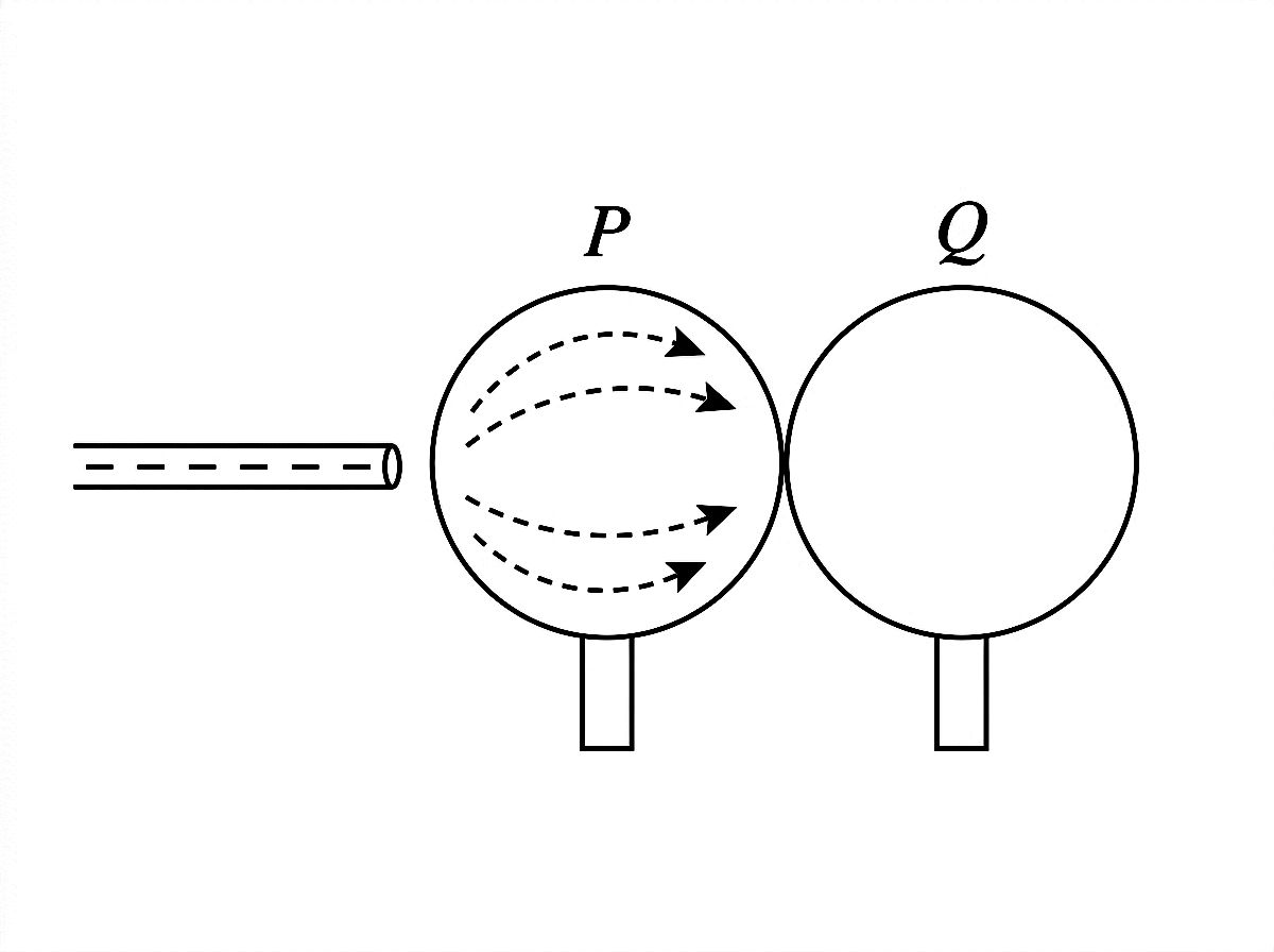
Step 1: Charge, force, and charging methods (Topics 10.1-10.2)Read the topic guides for 10.1 and 10.2. Practice applying Coulomb's law to two- and three-charge configurations, paying attention to direction. Then work through examples of charging by friction, contact, and induction, verifying charge conservation in each case. Use the electroscope as a concrete model for detecting charge redistribution.
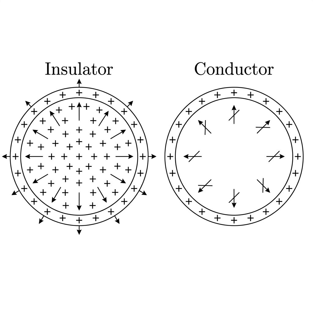
Step 2: Electric fields and field maps (Topic 10.3)Read the topic guide for 10.3. Practice sketching field vector maps and field line diagrams for single charges, dipoles, and parallel plates. Confirm you can apply vector superposition to find the net field at a point, and state the field rules for conductors and insulators in equilibrium.
Step 3: Potential energy and electric potential (Topics 10.4-10.5)Read the topic guides for 10.4 and 10.5. Work through pairwise U_E calculations for two- and three-charge systems, then practice scalar superposition for V. Draw equipotential maps from field maps and extract average field magnitudes using |E| = |delta V / delta r|. Focus on the sign conventions for both U_E and V.
Step 4: Capacitors (Topic 10.6)Read the topic guide for 10.6. Practice using C = Q/delta V and C = kappa epsilon_0 A/d to predict how changing plate area, gap, or dielectric affects C, Q, delta V, and stored energy. Work through at least one problem where the capacitor is disconnected from a battery before a change is made.
Step 5: Conservation of electric energy and full-unit review (Topic 10.7)Read the topic guide for 10.7. Practice delta U_E = q delta V and delta K = -delta U_E for both positive and negative charges moving through potential differences. Then use the available practice questions to work across all seven topics, and use the AP score calculator to estimate your estimated score range.

More ways to review

Topic study guides

Open the individual guides for Unit 10 when you want a closer review of one topic.

browse guides

Practice questions

Use AP-style practice after you review the notes so you can check what you understand.

start practice

FRQ practice

Practice free-response reasoning and compare your answer with scoring guidance.

practice FRQs

Cheatsheets

Use unit cheatsheets for a quick visual review after you work through the notes.

open cheatsheets

Score calculator

Estimate your broader AP score goal after you review the course and exam format.

open calculator

Frequently Asked Questions

What topics are covered in AP Physics 2 Unit 10?

AP Physics 2 Unit 10 covers 7 topics: Electric Charge and Electric Force, Conservation of Electric Charge and the Process of Charging, Electric Fields, Electric Potential Energy, Electric Potential, Capacitors, and Conservation of Electric Energy. Together they build from basic charge interactions up through energy storage in electric fields. See the full topic breakdown at AP Physics 2 Unit 10.

How much of the AP Physics 2 exam is Unit 10?

AP Physics 2 Unit 10 makes up 15-18% of the AP exam, making it one of the heavier-weighted units. It covers electric charge, electric force, electric fields, electric potential, capacitors, and conservation of electric energy, so strong performance here has a real impact on your overall score.

What's on the AP Physics 2 Unit 10 progress check (MCQ and FRQ)?

The AP Physics 2 Unit 10 progress check includes both MCQ and FRQ parts drawn from all 7 unit topics. The MCQ section tests concepts like electric charge, electric force, electric fields, and electric potential. The FRQ part asks you to apply those ideas quantitatively, often involving capacitors or conservation of electric energy. Practice with matched questions at AP Physics 2 Unit 10.

How do I practice AP Physics 2 Unit 10 FRQs?

AP Physics 2 Unit 10 FRQs most often pull from electric potential, electric fields, and capacitors. Questions typically ask you to derive or calculate quantities, draw or interpret field diagrams, and explain energy relationships using conservation of electric energy. To practice, work through problems that require you to connect multiple topics, like linking electric potential energy to capacitor charge storage, then check your reasoning step by step. Find practice FRQs at AP Physics 2 Unit 10.

Where can I find AP Physics 2 Unit 10 practice questions?

For AP Physics 2 Unit 10 practice questions, including multiple-choice and practice test sets, head to AP Physics 2 Unit 10. You'll find MCQs covering electric charge, electric force, electric fields, electric potential, and capacitors, plus full practice test questions organized by topic so you can target weak spots.

How should I study AP Physics 2 Unit 10?

Start with electric charge and electric force so Newton's laws feel familiar in an electrostatics context, then build toward electric potential and capacitors. Sketch field diagrams for every scenario you encounter. Practice moving between force, field, potential energy, and electric potential, since AP Physics 2 Unit 10 FRQs often require all four in one problem. After each topic, do a short set of MCQs to catch gaps early, then revisit conservation of electric energy last since it ties everything together. Organize your review at AP Physics 2 Unit 10.

Ready to review Unit 10?Start with the notes, check the topic cards, and use the practice or resource links when they are available for this course.