🎒ACT Review

Qualitative data describes non-numerical qualities or categories. For example, surveying teenagers about their favorite ice cream flavor produces qualitative data because the responses are categories (chocolate, vanilla, strawberry), not numbers.

Quantitative Data

Quantitative data is collected as numbers you can measure or count. For example, recording the heights of students in a high school produces quantitative data.

Quantitative data breaks into two subtypes:

Discrete data can only take specific values. Shoe sizes are a good example: you can have size 7 or 7.5, but not 7.333. There are only certain values allowed.
Continuous data can take any value within a range. Weight is continuous because someone could weigh 200 lbs, 127.752 lbs, or anything in between.

How Data Can Be Collected

Surveys and censuses ask a sample of people specific questions to gain insight about a larger population. A census attempts to survey the entire population.
Observational studies observe subjects without manipulating anything. They can identify correlations but cannot establish cause and effect.
Experiments deliberately apply a treatment to subjects to establish a cause-and-effect relationship. The key difference from observational studies is that the researcher controls the conditions.

A good sample should:

Have an appropriate size proportional to the population
Be representative of the population
Be randomly selected

🔮 Hypotheses

A hypothesis is a prediction about the outcome of a study. There are two types:

The null hypothesis ( $H_0$ ) claims there is no significant relationship between the variables being studied.
The alternative hypothesis ( $H_a$ ) predicts that a significant relationship does exist.

Here are some examples:

Null: There is no relationship between height and age among children.
Alternative: There is a relationship between height and age among children.
Null: There is no relationship between temperature and number of ice cream cones sold daily.
Alternative: The higher the temperature, the more ice cream cones sold in a day.

Significance Level

Once you have your hypotheses, you need to set a significance level (written as $\alpha$ ) before collecting data.

The significance level represents the maximum probability you're willing to accept of incorrectly claiming a relationship exists when it actually doesn't.
It's a threshold for how confident you need to be before rejecting the null hypothesis.
The lower the significance level, the stricter your standard for evidence.
For example, $\alpha = 0.07$ means you'll accept up to a 7% chance of falsely claiming a relationship exists.

P-Value

The p-value is calculated after data is collected.

It measures the probability of getting your observed results (or more extreme results) if the null hypothesis were actually true.
A lower p-value means stronger evidence against the null hypothesis.
P-values range from 0 to 1.
A very common significance level used is 0.05.

P-Value vs. Significance Level

The decision rule is straightforward:

If $p \leq \alpha$ : Reject the null hypothesis. Your data provides enough evidence to support a relationship between the variables.
If $p > \alpha$ : Fail to reject the null hypothesis. Your data doesn't provide strong enough evidence.

Examples:

$\alpha = 0.05$ and $p = 0.07$ → Cannot reject the null hypothesis ( $p > \alpha$ )
$\alpha = 0.01$ and $p = 0.01$ → Can reject the null hypothesis ( $p = \alpha$ )
$\alpha = 0.07$ and $p = 0.06$ → Can reject the null hypothesis ( $p < \alpha$ )

⌦ Errors

This section covers issues that can affect the accuracy of study results.

Bias

Bias is any factor that causes data to misrepresent the true population. Three common types appear on the ACT:

Nonresponse bias occurs when certain people choose not to respond to a survey, and those non-respondents differ systematically from respondents. For example, in a survey about GPA, students with lower GPAs may be less likely to respond, making the average GPA appear higher than it actually is.
Response bias results from the way a question is worded (leading questions) or from respondents answering dishonestly. For example, asking "Don't you agree that our school lunch is terrible?" pushes people toward a particular answer.
Under-coverage bias happens when a sample doesn't represent the full population. If you're studying how Americans do their grocery shopping but only survey people in Kentucky, the results won't generalize to the whole country.

Reducing Bias:

Sample a larger group of people
Include a more diverse group in the sample
Write neutral, unbiased questions
Increase anonymity of the survey

False Positives and Negatives

False Positive (Type I Error)

Concluding that something is true when it is actually false.
Example: A flu test says you have the flu, but you actually don't.
The probability of a Type I error equals $\alpha$ (the significance level).

False Negative (Type II Error)

Concluding that something is false when it is actually true.
Example: A blood pressure test says you don't have high blood pressure, but you actually do.
The probability of a Type II error is represented by $\beta$ (beta).

Inaccurate results can have serious consequences, especially in science and healthcare.

Power

Power is the probability that a test correctly rejects a false null hypothesis (i.e., it correctly detects a real relationship).
The formula is: $\text{Power} = 1 - \beta$
Higher power means a more reliable test.
Power can be increased by:
- Increasing sample size
- Increasing the significance level

📊 Center and Spread

🎯 Center

Three measures identify the center of a data set:

Mean is the average. Add all values and divide by the count.

$\text{Mean} = \frac{\text{sum of values}}{\text{number of values}}$

Example: Find the mean of {24, 9, 0, 0, 56, 9, 12, -7}

Sum the values: $24 + 9 + 0 + 0 + 56 + 9 + 12 + (-7) = 103$
Count the terms (include repeats and zeros): 8 terms
Divide: $103 / 8 = 12.875$

The mean is 12.875. Mean can also be represented by the Greek letter $\mu$ (mu).

Median is the middle value when data is arranged in order.

Arrange data points from smallest to largest.
Cross off the smallest and largest values in pairs, working inward.
If one value remains, that's the median. If two values remain, average them.

Example: Find the median of {30, 7, 89, 18, 4}

Order the values: 4, 7, 18, 30, 89
Cross off outer pairs: 4, 7, 18, 30, 89
The median is 18.

A data set with an even number of values will always have two middle values that need to be averaged.

Mode is the value that appears most often.

Not all data sets have a mode, and some have more than one.

Example: Find the mode of {9, 4, 7, 9, 10, 15, 7, 8, 4, 9, 9, 18}

9 appears four times, 4 appears twice, 7 appears twice, everything else appears once.
The mode is 9.

🌤 Advantages and Disadvantages

Mean

Works well when data has no strong skews or outliers.
Outliers pull the mean toward them. For example, in {1, 6, 3, 5, 2, 7, 566}, the mean is artificially high because of 566. The mean alone would give a misleading picture of this data.

Median

Stays reliable even with skewed data or outliers, since it only depends on position.
The downside is that it doesn't reflect how spread out the data is. For example, in {-56, -9, 0, 1, 1, 2, 3, 3, 3, 4, 7, 7, 45, 67, 89, 100, 2578, 99785}, the median is 3.5, which doesn't reveal the enormous range.

⭐️ When a data set is perfectly symmetrical, the mean and median are equal.

Spread 🍯

Spread (or variability) describes how spread out the values in a data set are.

High variability example: {-957, -350, -312, -177, -94, -84, -73, -20, 0, 1, 35, 52, 77, 100, 644, 981}
Low variability example: {-1, -0.5, -0.25, -0.1, 0, 0.2, 0.333, 0.6, 0.8, 1, 2, 2.5}

Range is the simplest measure of spread: subtract the smallest value from the largest.

Example: Range of {3, 4, 73, 95} → $95 - 3 = 92$
Example: Range of {-4, 9, 16, 22} → $22 - (-4) = 26$

Interquartile Range (IQR) measures the spread of the middle 50% of data.

Find the median of the full data set.
Split the data into lower and upper halves at the median.
Find the median of each half. The lower median is Q1 and the upper median is Q3.
$\text{IQR} = Q3 - Q1$

Example: IQR of {19, 23, 24, 26, 29, 33, 34}

Median of the full set: 26
Lower half: {19, 23, 24, 26} → median = $(23 + 24)/2 = 23.5$ (Q1)
Upper half: {26, 29, 33, 34} → median = $(29 + 33)/2 = 31$ (Q3)
$\text{IQR} = 31 - 23.5 = 7.5$

IQR is often used to create box and whisker plots.

Image Courtesy of Statistics Canada.

Standard Deviation ( $\sigma$ , sigma) measures the average distance of data points from the mean.

Greater standard deviation = more variability in the data.
You won't need to calculate standard deviation on the ACT, but you do need to understand what it represents and how to compare standard deviations between data sets.

💡 Tips and Tricks

Many of these concepts may feel familiar, so pay close attention to detail. Small arithmetic errors are the most common way to lose points here.
Practice with your actual test-day calculator so the process feels automatic.

Let's Practice!

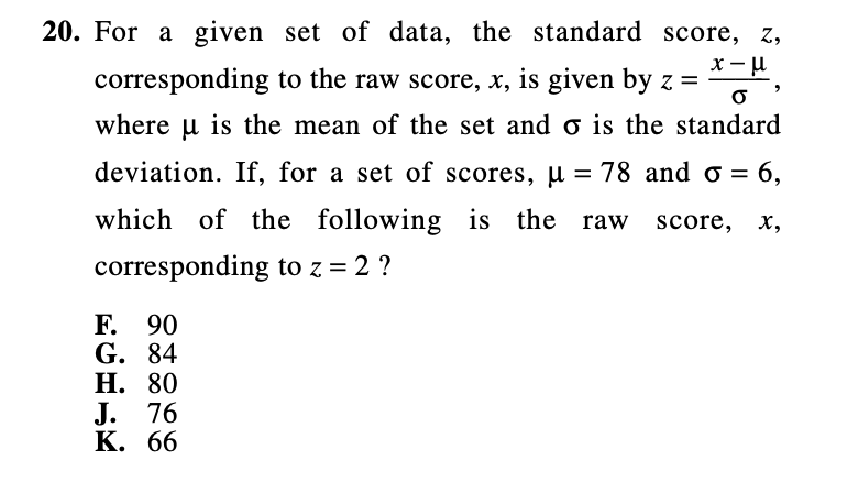
Image Courtesy of Preparing for the ACT Test 2023-2024.

This question asks you to rearrange the z-score equation to solve for $x$ . The z-score formula is:

$z = \frac{x - \mu}{\sigma}$

Multiply both sides by $\sigma$ : $z \cdot \sigma = x - \mu$
Add $\mu$ to both sides: $x = z \cdot \sigma + \mu$
Plug in the values: $x = 2(6) + 78 = 12 + 78 = 90$

The answer is F) 90

📈 Bivariate Data

Bivariate data compares two variables to see how they relate to each other.

Independent variable (x) represents the cause or input.
Dependent variable (y) represents the effect or output.

Examples:

Temperature outside (independent) vs. amount of ice cream melted (dependent). Temperature is the cause; melting is the effect.
Amount of cheese eaten daily (independent) vs. a person's weight (dependent). Cheese consumption is the potential cause; weight change is the effect.

📉 Correlation

Correlation describes the direction and strength of a relationship between two variables.

Correlation does not equal causation.

Three types of correlation:

Positive correlation (toward +1): As one variable increases, the other increases too. Example: More gas in the tank → greater distance the car can travel.
Negative correlation (toward -1): As one variable increases, the other decreases. Example: More time sleeping in class → lower grade.
No correlation (near 0): No relationship between the variables. Example: Number of penguins has no effect on croissants sold at a bakery.

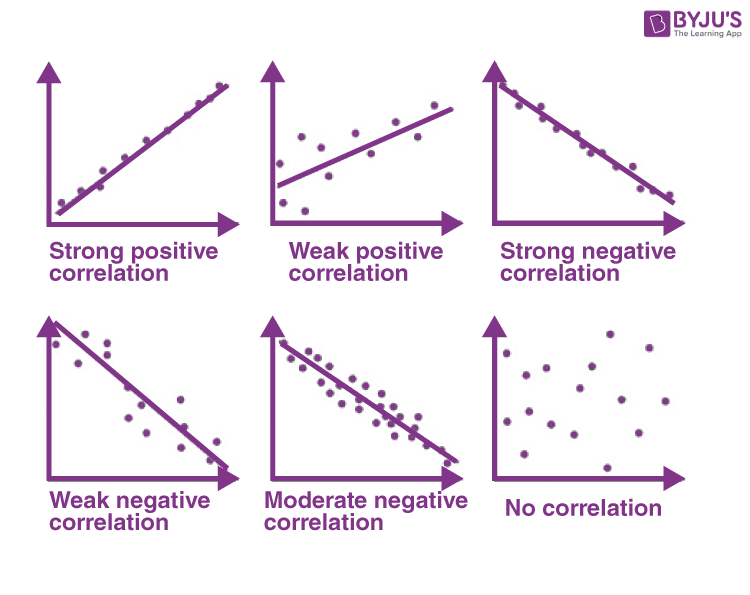
Image Courtesy of BYJU's

The correlation coefficient (often written as $r$ ) is a number from -1 to 1 that quantifies correlation:

Closer to -1 = stronger negative correlation
Closer to +1 = stronger positive correlation
Closer to 0 = weaker or no correlation

Practice

A correlation coefficient of 0.33 indicates a ______________ correlation.

A) Weak positive B) Strong positive C) Weak negative

Answer: A. Since 0.33 is positive, the correlation is positive. Since 0.33 is closer to 0 than to +1, it's a weak positive correlation.

A correlation coefficient of -0.75 indicates a _______________ correlation.

A) Weak positive B) Strong negative C) Weak negative

Answer: B. Since -0.75 is negative, the correlation is negative. Since -0.75 is closer to -1 than to 0, it's a strong negative correlation.

✨ Tips and Tricks

Create a quick memory device for interpreting correlation coefficients. You can jot it down on scratch paper at the start of the test.
Practice identifying correlation direction and strength from scatter plots. Many ACT questions on this topic include graphs.

🎊 More Practice

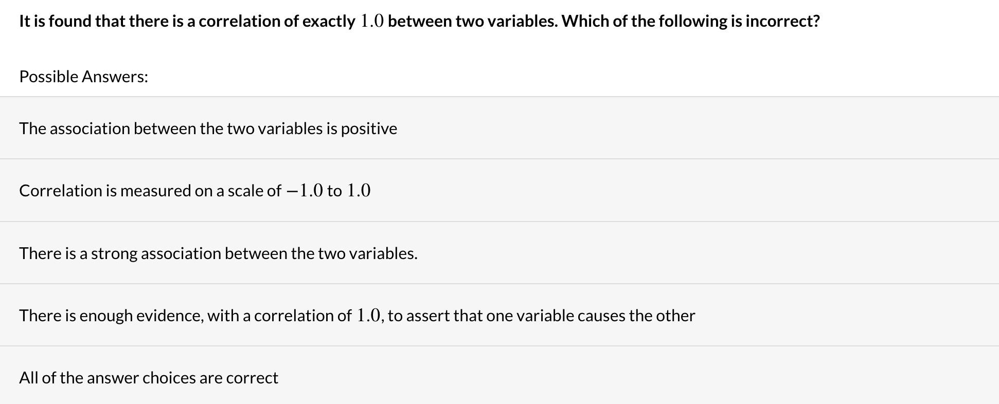
Image Courtesy of Varsity Tutors.

A correlation coefficient of 1.0 shows a perfect positive correlation, but it does not prove cause and effect. With that in mind, check each answer choice:

The association is positive → true, so eliminate.
Correlation is measured on a scale from -1 to +1 → true, so eliminate.
There is a strong correlation → true (1.0 is the strongest possible), so eliminate.
One variable causes the other → false. Correlation and causation are not the same thing. A correlation coefficient, no matter how strong, cannot prove that one variable causes changes in the other.

The answer is the fourth choice.

🎲 Simple Probabilities and Calculations

Standard Probability

Probability measures how likely an event is to occur, expressed as a fraction, decimal, or percentage.

$P(\text{event}) = \frac{\text{number of favorable outcomes}}{\text{total number of possible outcomes}}$

Example: A bag contains 10 blue marbles, 4 green marbles, and 3 yellow marbles. What's the probability of drawing a yellow marble?

Total marbles: $10 + 4 + 3 = 17$
Yellow marbles: 3
Probability: $\frac{3}{17} \approx 17.6\%$

"And" vs. "Or" Probability

"And" probability asks for the chance of one outcome AND another both happening. Multiply the individual probabilities.

Example: A pizza has 14 slices. 8 have pineapple, 10 have sardines, and 3 have olives. If you randomly pick one slice, what's the probability it has pineapple AND sardines?

Note: This problem assumes the toppings are distributed independently.

$P(\text{pineapple}) = \frac{8}{14}$
$P(\text{sardines}) = \frac{10}{14}$
$P(\text{both}) = \frac{8}{14} \times \frac{10}{14} = \frac{80}{196} \approx 40.8\%$

"Or" probability asks for the chance of one outcome OR another happening. Add the individual probabilities (for mutually exclusive events).

Example: A variety pack has 8 barbecue bags, 3 sour cream and onion bags, and 6 ketchup bags. What's the probability of randomly picking barbecue OR ketchup?

Total bags: $8 + 3 + 6 = 17$
$P(\text{barbecue}) = \frac{8}{17}$
$P(\text{ketchup}) = \frac{6}{17}$
$P(\text{barbecue or ketchup}) = \frac{8 + 6}{17} = \frac{14}{17} \approx 82.4\%$

Repeated Independent Events

When the same event can happen multiple times independently, multiply the probability by itself for each repetition.

Example: A teacher has 8 popsicle sticks with student names. After drawing a stick, it goes back in the bag. What's the probability of drawing Helen's name 5 times in a row?

Probability of drawing Helen once: $\frac{1}{8}$
Five times in a row (with replacement): $\left(\frac{1}{8}\right)^5 = \frac{1}{32768} \approx 0.003\%$

Sequential Events Without Replacement

When items are removed after selection, the total number of outcomes decreases each time.

Example: Same 8 sticks, but now each stick is removed after being drawn. What's the probability of choosing Liam, then Robert, then Helen in that exact order?

$P(\text{Liam first}) = \frac{1}{8}$
$P(\text{Robert second}) = \frac{1}{7}$ (7 sticks remain)
$P(\text{Helen third}) = \frac{1}{6}$ (6 sticks remain)
$P(\text{all three in order}) = \frac{1}{8} \times \frac{1}{7} \times \frac{1}{6} = \frac{1}{336} \approx 0.3\%$

🍡 Combinations and Permutations

Permutations: Order matters. Choosing A then B is different from B then A.
Combinations: Order does not matter. Choosing A and B is the same as choosing B and A.

The goal with both is to count how many different arrangements or groups are possible.

Permutations

Repeating Permutations (same option can be used more than once):

$\text{Total permutations} = n^r$

where $n$ = number of options and $r$ = number of positions to fill.

Example: How many 6-digit phone passcodes are possible (digits 0-9, repeats allowed)?

$10^6 = 1{,}000{,}000$ possible passcodes.

Non-Repeating Permutations (each option can only be used once):

$P(n, r) = \frac{n!}{(n - r)!}$

A factorial (written as $n!$ ) means multiplying a number by every positive integer below it. For example, $5! = 5 \times 4 \times 3 \times 2 \times 1 = 120$ . By definition, $0! = 1$ .

Example: How many 6-digit passcodes if no digit can repeat?

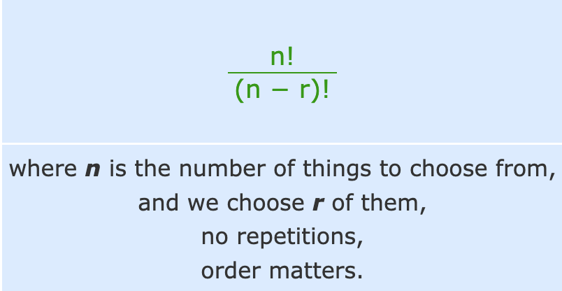
$\frac{10!}{(10-6)!} = \frac{10!}{4!} = 10 \times 9 \times 8 \times 7 \times 6 \times 5 = 151{,}200$

Image Courtesy of Math is Fun.

Combinations

Repeating Combinations (order doesn't matter, items can repeat):

$C(n + r - 1, r) = \frac{(n + r - 1)!}{r!(n - 1)!}$

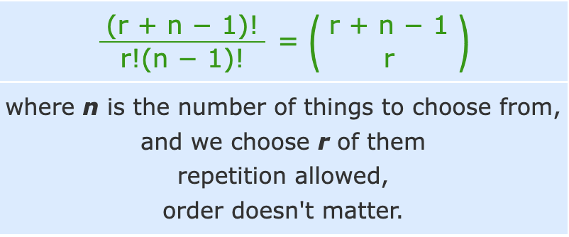
Image Courtesy of Math is Fun.

Example: You need to buy 2 cartons of milk from 4 options (low-fat, almond, soy, full-fat). You can buy two of the same kind. How many combinations?

$r = 2$ , $n = 4$
$\frac{(2 + 4 - 1)!}{2!(4 - 1)!} = \frac{5!}{2! \times 3!} = \frac{120}{2 \times 6} = 10$

10 possible combinations.

Non-Repeating Combinations (order doesn't matter, no repeats):

$C(n, r) = \frac{n!}{r!(n - r)!}$

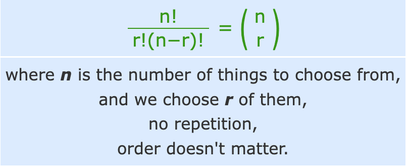
Image Courtesy of Math is Fun.

Example: You have 7 fruits/vegetables and want to pick 5 for a smoothie (no repeats). How many combinations?

$n = 7$ , $r = 5$
$\frac{7!}{5! \times 2!} = \frac{5040}{120 \times 2} = \frac{5040}{240} = 21$

21 possible combinations.

Tips and Tricks

Get comfortable with the formulas and practice using your calculator for factorials. Most scientific and graphing calculators have a factorial button.
Use the same calculator model for practice that you'll bring on test day.
If a problem looks complex, identify whether it's a permutation or combination first, then determine if repetition is allowed. That narrows you to one formula.
There is no penalty for guessing on the ACT. If you're stuck, eliminate what you can and pick an answer.

Let's Practice!

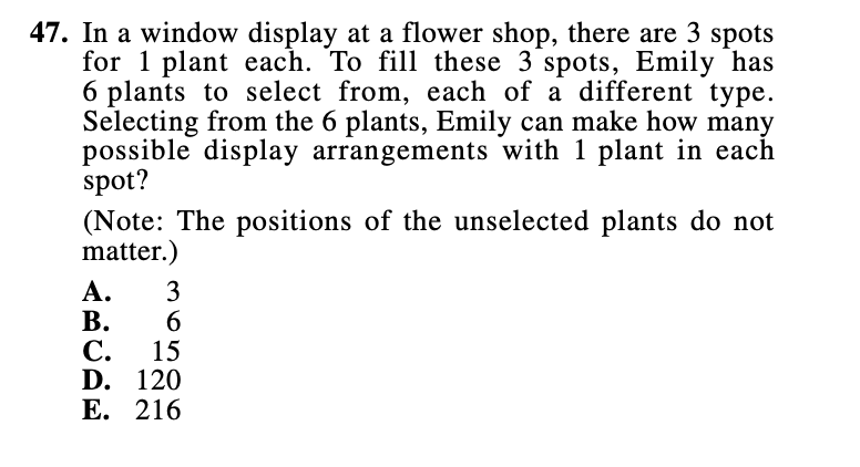
Image Courtesy of Preparing for the ACT Test 2023-2024.

This is a non-repeating permutation problem. Emily can't pick the same plant twice, and the order matters because each spot in the window is a distinct position.

Identify values: $n = 6$ plants, $r = 3$ spots
Apply the formula: $P(6, 3) = \frac{6!}{(6-3)!} = \frac{6!}{3!}$
Calculate: $\frac{6 \times 5 \times 4 \times 3!}{3!} = 6 \times 5 \times 4 = 120$

The answer is D) 120

📝 Quick Reference: Choosing the Right Formula

Scenario	Order Matters?	Repeats Allowed?	Formula
Repeating Permutation	Yes	Yes	$n^r$
Non-Repeating Permutation	Yes	No	$\frac{n!}{(n-r)!}$
Repeating Combination	No	Yes	$\frac{(n+r-1)!}{r!(n-1)!}$
Non-Repeating Combination	No	No	$\frac{n!}{r!(n-r)!}$

Let's Practice!

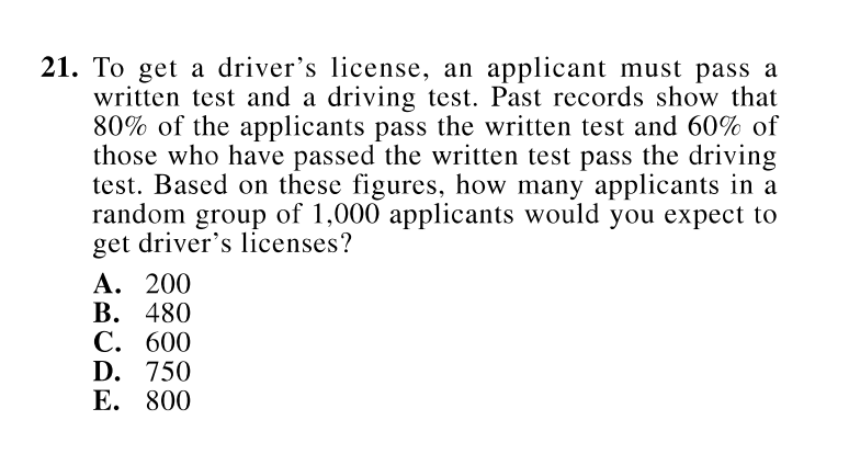
Image Courtesy of ACT Form 15AA51.

This question uses past data to predict outcomes for a group of 1,000 random applicants. Since the group is random, you can apply the same historical percentages.

Find how many pass the written test: $1000 \times 0.80 = 800$
Of those 800, find how many also pass the driving test: $800 \times 0.60 = 480$

The answer is B) 480

🎒ACT Review