9.1 Seasonal differencing and SARIMA models

Seasonal Differencing and SARIMA Models

Many real-world time series have recurring patterns tied to a calendar cycle: retail sales spike every December, electricity demand peaks every summer, and so on. Seasonal differencing and SARIMA models give you the tools to handle these repeating patterns. Seasonal differencing removes the predictable seasonal component so the data becomes stationary, and SARIMA models then capture whatever structure remains in both the short-term and seasonal behavior.

Seasonal Differencing in Time Series

Regular differencing (subtracting consecutive observations) removes trends. Seasonal differencing does something analogous but across seasonal periods: it subtracts the observation from the same season in the previous cycle. If you have monthly data, you subtract the value from 12 months ago. If you have quarterly data, you subtract the value from 4 quarters ago.

The notation looks like this:

$\nabla_s^D X_t = (1 - B^s)^D X_t$

Here, $s$ is the seasonal period (e.g., 12 for monthly data with an annual cycle), $D$ is the order of seasonal differencing, and $B^s$ is the backshift operator applied $s$ times (so $B^{12} X_t = X_{t-12}$).

Why do this? Stationarity is a key assumption for ARIMA-type models. If the data has a seasonal component that shifts over time, the series isn't stationary. Seasonal differencing strips out that component, leaving behind trend and irregular parts that you can handle with regular differencing and ARMA terms.

The order $D$ depends on how strong and persistent the seasonal pattern is. In practice, $D = 1$ handles the vast majority of cases. Higher orders are rare and can introduce unnecessary noise.

Structure of SARIMA Models

A SARIMA model extends ARIMA by adding a parallel set of seasonal parameters. The full notation is:

SARIMA$(p, d, q)(P, D, Q)_s$

The non-seasonal parameters work exactly like regular ARIMA:

• $p$: autoregressive (AR) order
• $d$: differencing order
• $q$: moving average (MA) order

The seasonal parameters mirror them but operate at multiples of the seasonal lag $s$:

• $P$: seasonal autoregressive (SAR) order
• $D$: seasonal differencing order
• $Q$: seasonal moving average (SMA) order
• $s$: the seasonal period itself

Seasonal autoregressive (SAR) component. This captures how the current observation depends on observations from previous seasonal cycles. Its polynomial is:

$\Phi_P(B^s) = 1 - \Phi_1 B^s - \Phi_2 B^{2s} - \cdots - \Phi_P B^{Ps}$

So with $P = 1$ and monthly data, the model says "this January depends partly on last January."

Seasonal moving average (SMA) component. This captures how the current observation depends on forecast errors from previous seasonal cycles:

$\Theta_Q(B^s) = 1 - \Theta_1 B^s - \Theta_2 B^{2s} - \cdots - \Theta_Q B^{Qs}$

With $Q = 1$ and monthly data, the model says "this January's value is partly influenced by how far off the forecast was last January."

The full SARIMA model multiplies the non-seasonal and seasonal polynomials together, which is how it captures interactions between short-term dynamics and seasonal behavior.

Determining the Order of Seasonal Differencing

Choosing the right value of $D$ is an important first step before fitting a SARIMA model. Here's how to approach it:

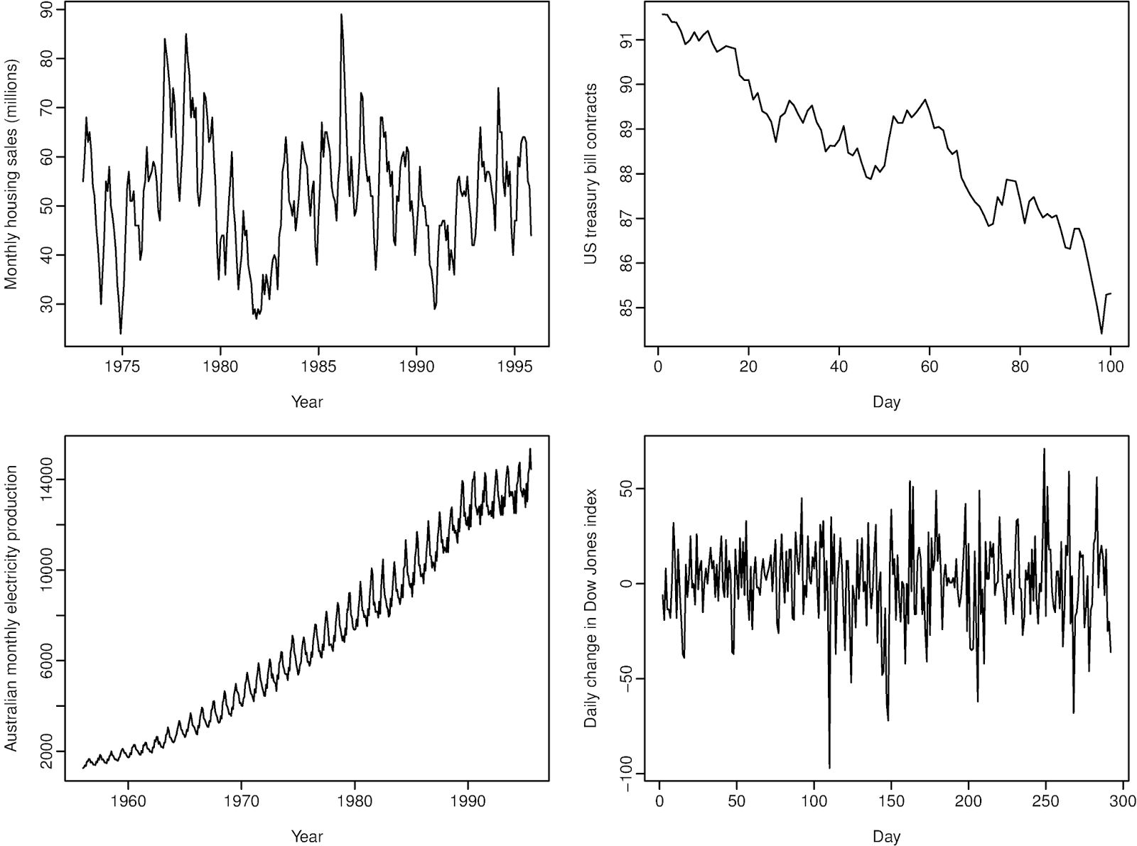
1. Plot the series and look at the seasonal swings over time.

   • If the seasonal pattern stays roughly the same amplitude year after year, you likely need $D = 0$ (no seasonal differencing).
   • If the seasonal swings grow or shrink proportionally with the level of the series, that suggests $D = 1$.

2. Check the ACF of the original series. If you see significant spikes at seasonal lags (lag 12, 24, 36 for monthly data) that decay very slowly, that's a strong signal you need seasonal differencing.

3. Apply seasonal differencing and re-examine. After taking $D = 1$, plot the differenced series and its ACF again. The slow seasonal decay should be gone. If it persists, you might need $D = 2$, but this is uncommon. Over-differencing can actually make things worse by introducing artificial patterns, so be cautious.

A useful rule of thumb: if the standard deviation of the series decreases after seasonal differencing, the differencing was likely appropriate. If it increases, you may have over-differenced.

Interpreting Seasonal ARIMA Terms

Once you've fit a SARIMA model, interpreting the seasonal coefficients tells you about the nature of the seasonal patterns in your data.

SAR coefficients ($\Phi_1, \Phi_2, \ldots, \Phi_P$) measure the strength and direction of the relationship between an observation and observations from previous seasonal cycles. A positive $\Phi_1$ close to 1 means this year's value for a given season strongly resembles last year's value for the same season. A negative coefficient would mean the series tends to alternate between high and low values across seasonal cycles.

SMA coefficients ($\Theta_1, \Theta_2, \ldots, \Theta_Q$) measure how forecast errors from past seasonal cycles influence the current value. These are often harder to interpret directly, but they play a critical role in capturing seasonal autocorrelation structure, especially when the ACF shows a sharp cutoff at seasonal lags rather than a slow decay.

Assessing significance. You evaluate whether each coefficient matters using t-tests or confidence intervals, just like with regular ARIMA terms. If a seasonal coefficient is not statistically significant, that term may not be contributing meaningfully to the model, and you should consider removing it for a more parsimonious fit. Comparing models with and without the term using AIC or BIC can also guide this decision.