Time series regression often faces , where error terms are linked across time periods. This can lead to issues with OLS estimators, including underestimated standard errors and inflated R-squared values, affecting hypothesis tests and forecasts.

(GLS) offers a solution by transforming the model to account for autocorrelation. This method estimates parameters more efficiently, yielding unbiased estimates and correct standard errors, which allows for valid inference and improved model fit.

Autocorrelated Errors in Time Series Regression

Autocorrelation in time series regression

Top images from around the web for Autocorrelation in time series regression
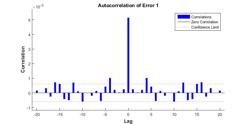
  • Error terms correlated with each other across time in a time series regression model
    • Positive autocorrelation: Errors tend to have the same sign as errors in the previous period (stock prices)
    • Negative autocorrelation: Errors tend to have the opposite sign as errors in the previous period (temperature fluctuations)
  • Consequences of autocorrelated errors lead to issues with OLS estimators
    • No longer the best linear unbiased estimators BLUE
    • Underestimated standard errors of coefficients result in invalid hypothesis tests and confidence intervals (t-tests, F-tests)
    • Inflated R-squared values give a false sense of model fit (spurious regression)
    • Inaccurate predictions and forecasts based on the model (weather forecasting, stock market predictions)

Generalized least squares for autocorrelation

  • Method to estimate parameters of a linear regression model with autocorrelated errors
    • Transforms model to account for autocorrelation structure in errors
    • Transformed model satisfies assumptions of classical linear regression model (homoscedasticity, no autocorrelation)
  • Applying GLS involves multiple steps
    1. Estimate autocorrelation structure of errors using residuals from OLS regression ()
    2. Transform original data using estimated autocorrelation structure ()
    3. Estimate regression model using transformed data
  • Yields efficient and unbiased parameter estimates in presence of autocorrelated errors (improved statistical properties)

Estimation and Interpretation of GLS Models

Estimation of GLS models

  • Obtain transformed data based on estimated autocorrelation structure
  • Apply OLS to transformed data to estimate model parameters
  • Interpret GLS model parameters
    • Coefficients represent change in dependent variable for one-unit change in independent variable, holding other variables constant
    • Interpretation similar to OLS, but coefficients adjusted for autocorrelation in errors (weather patterns, stock returns)
  • Hypothesis tests and confidence intervals for GLS model parameters
    • Use standard errors of coefficients from GLS estimation
    • Interpret results the same as OLS, but estimates adjusted for autocorrelation (t-tests, p-values)

OLS vs GLS for autocorrelated errors

  • OLS performance with autocorrelated errors
    • Estimates unbiased but inefficient
    • Underestimated standard errors lead to invalid inference (t-tests, confidence intervals)
    • Inflated R-squared values
  • GLS performance with autocorrelated errors
    • Estimates unbiased and efficient
    • Correctly estimated standard errors allow for valid inference
    • R-squared values not inflated, provide more accurate measure of model fit
  • Comparing OLS and GLS
    • GLS outperforms OLS with autocorrelated errors, providing more accurate and efficient estimates (economic models, climate data)
    • OLS used when errors not autocorrelated, simpler to implement and interpret (cross-sectional data)

Key Terms to Review (13)

Autocorrelated errors: Autocorrelated errors occur when the residuals or errors from a regression model are correlated with each other, meaning that the error terms are not independent. This violation of the assumption of independence can lead to inefficient estimates and unreliable statistical inferences, which is particularly problematic in time series data where observations are often related to previous values. Recognizing and addressing autocorrelation is crucial for producing valid regression results and ensuring accurate predictions.
Breusch-Godfrey Test: The Breusch-Godfrey test is a statistical procedure used to detect the presence of autocorrelation in the residuals of a regression model. This test is essential for validating the assumptions of ordinary least squares regression, particularly when errors are correlated over time, which can lead to inefficient estimates and invalid statistical inference. By identifying autocorrelation, the Breusch-Godfrey test helps in applying appropriate remedies, like generalized least squares, to correct for such issues.
Cochrane-Orcutt Procedure: The Cochrane-Orcutt procedure is a statistical method used to address the issue of autocorrelated errors in regression models by transforming the data. This procedure allows researchers to correct for the bias in standard ordinary least squares (OLS) estimates that arises when residuals are correlated, which can lead to inefficient and unreliable results. By applying this method, one can obtain more accurate parameter estimates and improve the overall effectiveness of the model.
Durbin-Watson Test: The Durbin-Watson test is a statistical test used to detect the presence of autocorrelation in the residuals from a regression analysis. This test helps identify whether the residuals are correlated, which is crucial for ensuring that the assumptions of regression analysis are met. Autocorrelation can lead to inefficient estimates and misleading statistical inference, so the Durbin-Watson test serves as an important diagnostic tool in regression with time series data.
Elasticity: Elasticity measures how much one variable responds to changes in another variable. In the context of statistical analysis, particularly in time series data, it reflects the sensitivity of the dependent variable to changes in independent variables. Understanding elasticity helps in assessing the robustness of relationships within models, especially when dealing with errors and inefficiencies in predictions.
Generalized Least Squares: Generalized Least Squares (GLS) is a statistical technique used to estimate the parameters of a linear regression model when the assumption of homoscedasticity (constant variance of the errors) is violated. This method is particularly useful when dealing with autocorrelated errors, which occur when the error terms are correlated across observations, potentially leading to inefficient estimates and biased standard errors. By incorporating a weighting matrix, GLS improves the efficiency of the estimates and provides more reliable hypothesis testing.
Independence: Independence refers to the condition in which two random variables or observations do not influence each other, meaning that the occurrence of one does not provide any information about the occurrence of the other. This concept is crucial for ensuring the validity of statistical models and inference, as violations can lead to misleading results, especially in the context of errors in time series analysis, model selection processes, and the evaluation of residuals.
Ljung-Box test: The Ljung-Box test is a statistical test used to determine whether any of a group of autocorrelations of a time series are different from zero, indicating that the time series is not white noise. This test plays a crucial role in assessing model adequacy, especially in regression contexts, and is also significant for time series forecasting and error analysis.
Marginal Effects: Marginal effects refer to the impact that a one-unit change in an independent variable has on the dependent variable in a statistical model. This concept is crucial for understanding how changes in predictors influence outcomes, especially in the presence of autocorrelated errors, where the standard errors can be biased, affecting inference and predictions derived from models like generalized least squares.
Normality: Normality refers to the statistical property of a distribution where the data points are symmetrically distributed around the mean, following a bell-shaped curve. In time series analysis, normality is crucial because many statistical methods, including hypothesis tests and regression analyses, assume that the residuals (errors) of a model are normally distributed to produce reliable results. A failure to meet this assumption can lead to biased estimates and incorrect conclusions.
Ordinary Least Squares: Ordinary Least Squares (OLS) is a statistical method used to estimate the relationships between variables by minimizing the sum of the squared differences between observed and predicted values. This technique is fundamental in regression analysis and provides a way to model relationships between dependent and independent variables, offering insights into how these variables interact. In contexts involving autocorrelated errors, OLS can yield biased estimates, making it essential to consider generalized least squares for more accurate modeling. Additionally, in Vector Autoregression models, OLS plays a critical role in estimating the coefficients that describe the dynamics among multiple time series.
Seasonality: Seasonality refers to periodic fluctuations in time series data that occur at regular intervals, often influenced by seasonal factors like weather, holidays, or economic cycles. These patterns help in identifying trends and making predictions by accounting for variations that repeat over specific timeframes.
Stationarity: Stationarity refers to a property of a time series where its statistical characteristics, such as mean, variance, and autocorrelation, remain constant over time. This concept is crucial for many time series analysis techniques, as non-stationary data can lead to unreliable estimates and misleading inferences.
© 2024 Fiveable Inc. All rights reserved.
AP® and SAT® are trademarks registered by the College Board, which is not affiliated with, and does not endorse this website.