10.3 Cointegration and error correction models

Cointegration and Error Correction Models

Cointegration helps you identify long-term equilibrium relationships between non-stationary time series. Two variables might each wander unpredictably on their own, but if they're cointegrated, they're tethered together over time. Error Correction Models (ECMs) then capture both the short-run dynamics and the mechanism that pulls variables back toward that long-run equilibrium.

Cointegration

Cointegration in Time Series

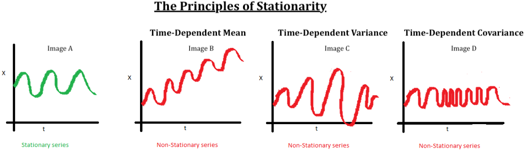
Two or more non-stationary time series are cointegrated if some linear combination of them produces a stationary series. In plain terms: each series individually has a unit root (trending mean, non-constant variance, etc.), but together they share a common stochastic trend and maintain a long-run equilibrium relationship.

• Deviations from this equilibrium are stationary and mean-reverting. Think of a stock price and its futures contract: they can diverge briefly, but the spread between them tends to snap back.
• Cointegrated series move together over the long run, preventing them from drifting arbitrarily far apart. Interest rates and inflation are a classic example.
• Because the equilibrium relationship is stable, you can estimate long-run parameters and measure how quickly variables adjust back to equilibrium after a shock.

The key distinction from ordinary correlation: correlation measures co-movement at a point in time, while cointegration describes a persistent structural relationship that holds across time, even when individual series are non-stationary.

Tests for Cointegrating Relationships

Engle-Granger Test — a two-step, residual-based approach:

1. Estimate the long-run equilibrium relationship using OLS: $y_t = \beta_0 + \beta_1 x_t + u_t$
2. Test the residuals $u_t$ for stationarity using a unit root test (typically the Augmented Dickey-Fuller test).
   • If $u_t$ is stationary, the series are cointegrated. For example, regressing household expenditure on income and finding stationary residuals would suggest cointegration.

This test is simple but limited to one cointegrating relationship between two variables.

Johansen Test — a maximum likelihood approach within a Vector Autoregressive (VAR) framework:

• Can test for multiple cointegrating relationships among several variables simultaneously (e.g., GDP, consumption, and investment).
• Works by examining the rank of the long-run coefficient matrix in the VAR. The rank tells you how many independent cointegrating vectors exist.
• Uses two test statistics: the trace statistic (tests whether the number of cointegrating vectors is at most $r$) and the maximum eigenvalue statistic (tests $r$ vs. $r+1$ cointegrating vectors).

Error Correction Models (ECMs)

Error Correction Models

An ECM captures both short-run fluctuations and the long-run equilibrium in a single equation. The general form for two cointegrated variables is:

$\Delta y_t = \alpha_0 + \alpha_1 \Delta x_t + \alpha_2 (y_{t-1} - \beta_0 - \beta_1 x_{t-1}) + \varepsilon_t$

Breaking this apart:

• $\Delta y_t$ and $\Delta x_t$ are first differences, capturing short-run dynamics (e.g., period-to-period changes in stock prices).
• $(y_{t-1} - \beta_0 - \beta_1 x_{t-1})$ is the error correction term. It measures how far the system was from equilibrium in the previous period. If the stock-futures spread was unusually wide last period, this term picks that up.

Estimating an ECM (Engle-Granger two-step method):

1. Estimate the long-run relationship $y_t = \beta_0 + \beta_1 x_t + u_t$ using OLS. Save the residuals $\hat{u}_t$.
2. Estimate the ECM using OLS, plugging in the lagged residuals $\hat{u}_{t-1}$ as the error correction term: $\Delta y_t = \alpha_0 + \alpha_1 \Delta x_t + \alpha_2 \hat{u}_{t-1} + \varepsilon_t$

Interpretation of ECM Parameters

• Short-run coefficient ($\alpha_1$): The immediate impact of a one-unit change in $x$ on $y$. For instance, how a sudden change in income affects consumption this period.
• Long-run coefficient ($\beta_1$): The equilibrium relationship between the variables. If $\beta_1 = 0.8$ in a consumption-income model, then in the long run, a one-unit increase in income is associated with a 0.8-unit increase in consumption.
• Adjustment parameter ($\alpha_2$): The speed at which $y$ corrects back toward equilibrium.
  • This value should be negative and statistically significant for a valid ECM. A negative sign means the system corrects toward equilibrium rather than away from it.
  • The larger the absolute value, the faster the adjustment. An $\alpha_2$ of $-0.5$ means about half of any disequilibrium is corrected each period, while $-0.1$ means only 10% is corrected per period.

Applications of ECMs

Forecasting: ECMs tend to produce more accurate forecasts than models that ignore cointegration, particularly over longer horizons. The error correction term anchors predictions to the long-run equilibrium, preventing forecasts from drifting unrealistically. Exchange rate forecasting is a common application.

Policy analysis: ECMs let you separate the short-run and long-run effects of a policy change or shock. For example, you could model how a tax cut affects consumption immediately (short-run coefficient) versus after the economy fully adjusts (long-run coefficient). The adjustment parameter tells you how quickly the system returns to equilibrium after the intervention.

Impulse response functions derived from ECMs trace out the dynamic path of how a shock propagates through the system over time. You can visualize, for instance, how inflation responds period-by-period to a monetary policy shock, and how long it takes for the effect to fade as the system returns to equilibrium.