16.1 Climate data analysis

Climate data analysis applies time series techniques to understand long-term trends and patterns in environmental datasets. These methods let researchers quantify warming trends, detect cyclical patterns like El Niño, and forecast future climate conditions, all of which feed directly into policy decisions and adaptation planning.

Climate Data Analysis Techniques

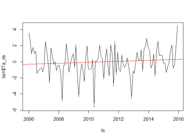
Time series analysis of climate trends

Three main approaches help you identify and measure trends in climate data: regression-based methods, smoothing techniques, and decomposition.

Trend Analysis

• Linear regression fits a straight line to the data using least squares. The slope tells you the direction and magnitude of the trend: a positive slope indicates warming, a negative slope indicates cooling.
• Mann-Kendall test is a non-parametric test for monotonic trends (consistent increase or decrease over time). Because it doesn't assume normality, it handles the outliers and extreme values common in climate data.
• Sen's slope estimator calculates the median slope among all pairs of data points. Taking the median rather than the mean makes it resistant to outliers, giving a more stable trend estimate than ordinary regression.

Smoothing Techniques

• Moving average reduces short-term fluctuations to highlight long-term trends. A 10-year moving average is common for climate data. Larger windows produce smoother curves; smaller windows preserve more detail.
• Exponential smoothing assigns exponentially decreasing weights to older observations, so recent data has more influence. This works well for data without a clear trend or seasonal pattern, such as temperature anomalies.

Decomposition Methods

Decomposition splits a time series into three components:

• $T_t$: the trend component (long-term direction)
• $S_t$: the seasonal component (recurring within-year pattern)
• $R_t$: the remainder/irregular component (unexplained variation)

The two standard forms are:

• Additive: $Y_t = T_t + S_t + R_t$
• Multiplicative: $Y_t = T_t \times S_t \times R_t$

Use additive decomposition when the seasonal swings stay roughly constant over time. Use multiplicative when the seasonal variation grows or shrinks proportionally with the trend.

Detection of climate data patterns

Once you've decomposed a series, several tools help you identify and characterize the cyclical patterns within it.

Seasonal decomposition isolates the seasonal component from the time series. Seasonal indices represent the average deviation from the trend for each season. For temperature data, summer months typically sit above the trend and winter months below.

Fourier analysis expresses the time series as a sum of sine and cosine waves. Each wave has a frequency and amplitude, so you can identify dominant cycles: annual, semi-annual, decadal, or others. This is particularly useful for detecting phenomena like the El Niño Southern Oscillation (ENSO), which operates on irregular multi-year cycles.

Autocorrelation function (ACF) measures the correlation between a time series and its own lagged values. Seasonal patterns show up as significant autocorrelation at seasonal lags. For example, January temperatures in consecutive years tend to be highly correlated.

Periodogram estimates spectral density, which is how variance is distributed across frequencies. Peaks in the periodogram point to dominant cycles. Temperature data, for instance, typically shows a strong peak at the annual frequency.

Statistical significance of climate trends

Detecting a trend visually isn't enough. You need to test whether it's statistically distinguishable from random noise.

Hypothesis testing follows the standard framework:

1. Set up the null hypothesis ($H_0$): no significant trend (slope equals zero).
2. Set up the alternative hypothesis ($H_a$): a significant trend exists (slope is non-zero).
3. Compute the p-value, which is the probability of observing data this extreme if $H_0$ were true.
4. Reject $H_0$ if the p-value falls below your significance level (typically 0.05).

Confidence intervals quantify uncertainty around the estimated trend. A 95% confidence interval gives a range of plausible values for the true trend. Narrow intervals mean more precise estimates; wide intervals signal more uncertainty, often due to high variability or limited data.

Bootstrap resampling is a non-parametric alternative that doesn't assume a specific distribution:

1. Resample the data with replacement to create many new datasets.
2. Calculate the trend for each resample.
3. Use the distribution of resampled trends to build confidence intervals (e.g., the 2.5th and 97.5th percentiles for a 95% interval).

This approach is especially valuable for climate data, where the underlying distribution may not be well-behaved.

Climate forecasting models from historical data

ARIMA models (Autoregressive Integrated Moving Average) combine three components: autoregressive (AR) terms that use past values, differencing (I) to remove trends and achieve stationarity, and moving average (MA) terms that use past forecast errors. Standard ARIMA works well for non-seasonal series like annual global temperature anomalies. Model selection typically relies on information criteria such as AIC or BIC, which balance model complexity against goodness of fit.

SARIMA models (Seasonal ARIMA) extend ARIMA by adding seasonal AR, differencing, and MA terms. This lets them capture both the long-term trend and recurring seasonal patterns. Monthly sea surface temperature data is a classic use case.

Exponential smoothing models offer a complementary approach:

• Holt-Winters method handles data with both trend and seasonality. You choose additive seasonality when seasonal swings are constant in magnitude, or multiplicative when they scale with the level.
• Damped trend models gradually flatten the trend over the forecast horizon. These are useful for long-term climate projections where assuming the current trend continues indefinitely would be unrealistic.

Model evaluation is critical for any forecasting approach:

1. Split the data into training and testing sets (e.g., 80/20).
2. Fit the model on the training set and generate forecasts for the test period.
3. Assess accuracy using metrics like RMSE (root mean squared error), MAE (mean absolute error), or MAPE (mean absolute percentage error).
4. For more robust evaluation, use cross-validation techniques like rolling origin forecasting, which repeatedly moves the train-test boundary forward through time. This reduces the risk that your results depend on one particular split.