Evaluating forecast accuracy tells you how well your model's predictions match reality. Without a reliable way to measure errors, you can't compare models, spot problems, or know whether your forecasts are actually useful for decisions like budgeting or inventory planning.
Three metrics show up constantly in practice: Mean Absolute Error (MAE), Root Mean Squared Error (RMSE), and Mean Absolute Percentage Error (MAPE). Each one captures forecast error differently, and knowing when to use which is just as important as knowing how to calculate them.
Evaluating Forecast Accuracy
Importance of forecast accuracy evaluation
Forecast accuracy evaluation isn't just a final checkbox. It's woven into every stage of building and maintaining a time series model.
- Model selection: Accuracy metrics help you pick the best model for your data (e.g., choosing between ARIMA and exponential smoothing based on which produces lower error on a holdout set).
- Diagnosing problems: Consistently high errors can reveal overfitting (model memorizes training data but fails on new data) or underfitting (model is too simple to capture the pattern).
- Supporting decisions: Forecasts drive real actions like staffing, purchasing, and budgeting. Knowing how wrong your forecasts tend to be lets decision-makers plan with appropriate caution.
- Ongoing monitoring: A model that worked well six months ago might degrade as underlying patterns shift. Tracking accuracy over time tells you when it's time to retrain or switch methods.

Mean Absolute Error calculation
MAE measures the average size of your forecast errors, ignoring their direction. It answers: on average, how far off are my predictions?
- = number of forecast periods
- = actual value at time
- = forecasted value at time
How to compute it step by step:
-
For each time period, subtract the forecast from the actual value: .
-
Take the absolute value of each difference (drop the sign).
-
Sum all the absolute differences.
-
Divide by (the number of observations).
Example: Suppose you forecast daily sales for 3 days. Actuals are 100, 150, 130 and forecasts are 110, 140, 135. The absolute errors are 10, 10, and 5. So units.
MAE is expressed in the same units as your data (dollars, units sold, etc.), which makes it straightforward to communicate. It's also less sensitive to outliers than RMSE because it doesn't square the errors. The tradeoff is that MAE treats a 1-unit error and a 50-unit error with equal weight per unit of error, which may not reflect the true cost of large misses.
Root Mean Squared Error computation
RMSE also measures average error magnitude, but it penalizes larger errors more heavily because it squares each error before averaging.
- = number of forecast periods
- = actual value at time
- = forecasted value at time
How to compute it step by step:
-
For each time period, calculate the error: .
-
Square each error.
-
Sum all the squared errors.
-
Divide by .
-
Take the square root of the result.
Using the same example: Errors are -10, 10, -5. Squared errors are 100, 100, 25. Mean of squared errors = 75. units.
Notice RMSE (8.66) is slightly higher than MAE (8.33) here. That gap widens when you have a few large errors mixed in with small ones, because squaring amplifies big misses. This property makes RMSE a better choice when large errors are especially costly (think financial risk or safety-critical applications). Like MAE, RMSE is in the same units as the data, but the squaring step makes it a bit less intuitive to explain to non-technical audiences.
Mean Absolute Percentage Error interpretation
MAPE converts errors into percentages of the actual values, making it scale-independent. This is useful when you need to compare accuracy across datasets measured in different units or magnitudes.
- = number of forecast periods
- = actual value at time
- = forecasted value at time
How to compute it step by step:
-
For each time period, calculate the error: .
-
Divide each error by the actual value .
-
Take the absolute value of each percentage error.
-
Sum all the absolute percentage errors.
-
Divide by and multiply by 100%.
Using the same example: Percentage errors are |−10/100|, |10/150|, |−5/130| = 0.10, 0.067, 0.038. .
A MAPE of 6.83% means your forecasts are off by about 6.83% on average. That's easy for stakeholders to grasp regardless of what the data measures.
The big limitation: MAPE divides by , so if any actual value is zero (or very close to zero), the metric blows up or becomes misleading. Avoid MAPE for data that naturally includes zeros (e.g., intermittent demand).
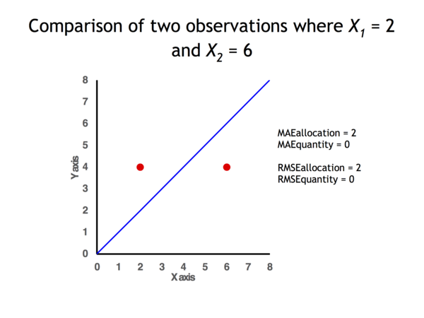
Comparison of accuracy measures
| MAE | RMSE | MAPE | |
|---|---|---|---|
| Units | Same as data | Same as data | Percentage |
| Outlier sensitivity | Lower | Higher (squaring amplifies large errors) | Depends on scale of actuals |
| Cross-scale comparison | Not ideal | Not ideal | Yes, scale-independent |
| Handles zeros in data | Yes | Yes | No (undefined when ) |
| Interpretability | Very intuitive | Slightly less intuitive | Intuitive as a percentage |
| Optimization-friendly | Less so (absolute value not differentiable at 0) | Yes (quadratic, differentiable) | Less so |
When to use which:
- MAE is your default go-to when you want a simple, robust summary of average error size and your data doesn't have extreme outlier concerns.
- RMSE is the better pick when large errors carry disproportionate costs, or when you're optimizing a model (many algorithms minimize squared error naturally).
- MAPE shines when you need to compare forecast quality across series with different scales (e.g., forecasting both a product that sells 50 units/day and one that sells 5,000 units/day), but only if your actuals stay well away from zero.
In practice, reporting more than one metric gives a fuller picture. If MAE and RMSE are close together, your errors are fairly uniform. If RMSE is much larger than MAE, a few big misses are pulling the average up, and that's worth investigating.