9.2 Elliptic curves and linear codes

Elliptic curves over finite fields are powerful tools in cryptography and coding theory. They provide a discrete algebraic structure that enables secure encryption and efficient error correction. Understanding their properties and arithmetic is crucial for implementing robust cryptographic systems and error-correcting codes.

Linear error-correcting codes add redundancy to data, allowing detection and correction of transmission errors. These codes, including Hamming and Goppa codes, use mathematical structures to achieve optimal error-correcting capabilities. Their applications span telecommunications, data storage, and cryptography.

Elliptic curves over finite fields

• Elliptic curves over finite fields play a fundamental role in cryptography and coding theory
• Finite fields provide a discrete and bounded algebraic structure for defining elliptic curves
• Understanding the properties and arithmetic of elliptic curves over finite fields is crucial for their applications

Definitions and examples

• An elliptic curve over a finite field $\mathbb{F}_q$ is defined by an equation of the form $y^2 = x^3 + ax + b$ where $a, b \in \mathbb{F}_q$ and the discriminant $\Delta = 4a^3 + 27b^2 \neq 0$
• The set of points $(x, y)$ satisfying the equation along with a special point at infinity denoted $\mathcal{O}$ form the elliptic curve
• Example: The curve $y^2 = x^3 + x + 1$ over the field $\mathbb{F}_5 = \{0, 1, 2, 3, 4\}$ consists of the points $\{(0, 1), (0, 4), (2, 1), (2, 4), (3, 1), (3, 4), \mathcal{O}\}$

Group law and point addition

• The set of points on an elliptic curve over a finite field forms an abelian group under a well-defined addition operation
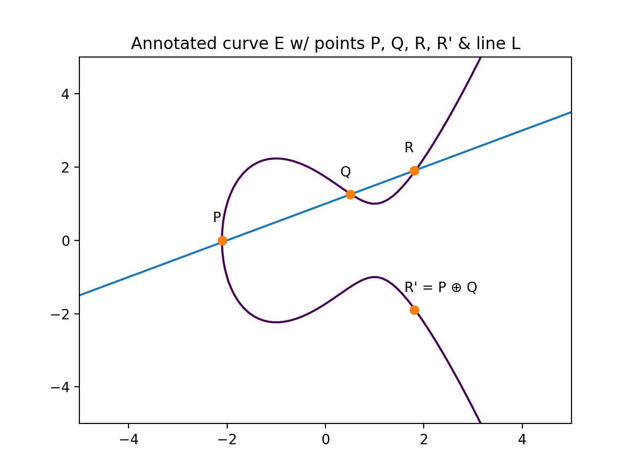
• The group law is based on the chord-and-tangent method for adding points geometrically
• Given two points $P$ and $Q$ on the curve, their sum $P + Q$ is defined as the reflection across the x-axis of the third point of intersection of the line through $P$ and $Q$ with the curve
• The point at infinity $\mathcal{O}$ serves as the identity element of the group
• Example: On the curve $y^2 = x^3 + x + 1$ over $\mathbb{F}_5$, the sum of points $(2, 1)$ and $(3, 4)$ is $(0, 4)$

Finite field arithmetic

• Elliptic curve operations involve arithmetic in the underlying finite field $\mathbb{F}_q$
• Finite field elements are represented as integers modulo the field size $q$
• Addition, subtraction, multiplication, and division in the finite field are performed modulo $q$
• Efficient algorithms exist for finite field arithmetic, such as Montgomery multiplication and fast modular reduction techniques
• Example: In $\mathbb{F}_5$, the sum of $2$ and $3$ is $0$ (since $2 + 3 \equiv 0 \pmod{5}$), and the product of $2$ and $3$ is $1$ (since $2 \times 3 \equiv 1 \pmod{5}$)

Singular vs non-singular curves

• A non-singular elliptic curve over a finite field has a non-zero discriminant and forms a smooth curve without any cusps or self-intersections
• Singular curves have a vanishing discriminant and possess singularities or points of self-intersection
• Cryptographic applications typically use non-singular curves to ensure desirable group properties and security
• Example: The curve $y^2 = x^3$ over $\mathbb{F}_5$ is singular at the point $(0, 0)$, while the curve $y^2 = x^3 + x + 1$ is non-singular

Linear error-correcting codes

• Linear error-correcting codes are mathematical constructions used for detecting and correcting errors in data transmission or storage
• They provide a systematic way to add redundancy to information symbols to enable error correction
• Linear codes are widely used in various applications, including telecommunications, data storage, and cryptography

Generator and parity check matrices

• A linear code $\mathcal{C}$ of length $n$ and dimension $k$ over a finite field $\mathbb{F}_q$ is a $k$-dimensional subspace of the vector space $\mathbb{F}_q^n$
• The generator matrix $G$ is a $k \times n$ matrix whose rows form a basis for the code $\mathcal{C}$
• The parity check matrix $H$ is an $(n-k) \times n$ matrix such that $GH^T = 0$, where $H^T$ denotes the transpose of $H$
• Codewords in $\mathcal{C}$ are obtained by multiplying a message vector $m \in \mathbb{F}_q^k$ with the generator matrix $G$, i.e., $c = mG$
• Example: The generator matrix $G = \begin{pmatrix} 1 & 0 & 1 & 1 \\ 0 & 1 & 1 & 2 \end{pmatrix}$ over $\mathbb{F}_3$ generates a $(4, 2)$ linear code

Hamming codes and perfect codes

• Hamming codes are a family of linear codes with parameters $[2^r - 1, 2^r - r - 1, 3]$ for any positive integer $r$
• They are single-error-correcting codes, capable of correcting any single-bit error in a codeword
• Perfect codes are codes that achieve the Hamming bound, meaning they have the maximum possible minimum distance for a given code length and dimension
• Hamming codes are perfect codes for the case of single-error correction
• Example: The $[7, 4, 3]$ Hamming code can correct any single-bit error in a 7-bit codeword

Bounds on minimum distance

• The minimum distance $d$ of a linear code determines its error-correcting capability
• The Singleton bound states that $d \leq n - k + 1$ for an $[n, k]$ linear code
• The Hamming bound provides an upper bound on the size of a code with a given minimum distance
• Codes meeting the Singleton bound are called maximum distance separable (MDS) codes
• Example: The $[7, 4, 3]$ Hamming code meets the Singleton bound and is an MDS code

Decoding algorithms for linear codes

• Decoding algorithms aim to correct errors in received codewords and recover the original message
• Syndrome decoding is a common technique that computes the syndrome of a received word and uses it to determine the error pattern
• Maximum likelihood decoding finds the codeword closest to the received word in terms of Hamming distance
• Algebraic decoding methods, such as the Berlekamp-Massey algorithm, use the algebraic structure of the code for efficient decoding
• Example: Syndrome decoding of the $[7, 4, 3]$ Hamming code can correct any single-bit error by comparing the syndrome with a pre-computed syndrome table

Goppa codes from algebraic curves

• Goppa codes are a class of linear error-correcting codes constructed from algebraic curves over finite fields
• They provide a geometric approach to coding theory and offer advantages over classical linear codes in terms of code parameters and decoding efficiency
• Goppa codes have found applications in cryptography, such as the McEliece cryptosystem, due to their resistance to certain cryptanalytic attacks

Goppa's construction from curves

• Goppa codes are constructed from a smooth, projective, absolutely irreducible algebraic curve $\mathcal{X}$ over a finite field $\mathbb{F}_q$
• Given a set of $n$ distinct $\mathbb{F}_q$-rational points $P_1, \ldots, P_n$ on $\mathcal{X}$ and a divisor $D$ on $\mathcal{X}$ with support disjoint from the $P_i$, the Goppa code $\mathcal{C}(P_1, \ldots, P_n, D)$ is defined as the image of the evaluation map from the Riemann-Roch space $\mathcal{L}(D)$ to $\mathbb{F}_q^n$
• The generator matrix of the Goppa code is constructed from the basis elements of $\mathcal{L}(D)$ evaluated at the points $P_i$
• Example: The Hermitian curve $y^q + y = x^{q+1}$ over $\mathbb{F}_{q^2}$ can be used to construct Goppa codes with good parameters

Parameters of Goppa codes

• The length $n$ of a Goppa code is determined by the number of $\mathbb{F}_q$-rational points used in the construction
• The dimension $k$ of the code is related to the dimension of the Riemann-Roch space $\mathcal{L}(D)$ and can be computed using the Riemann-Roch theorem
• The minimum distance $d$ of the code is lower bounded by the degree of the divisor $D$ used in the construction
• Example: A Goppa code constructed from the Hermitian curve over $\mathbb{F}_{16}$ with $n = 64$ and $\deg(D) = 24$ has parameters $[64, 18, \geq 25]$

Decoding Goppa codes

• Decoding Goppa codes involves finding the closest codeword to a received word in terms of Hamming distance
• Efficient decoding algorithms for Goppa codes exploit the algebraic structure of the code and the underlying curve
• The Patterson algorithm is a widely used decoding method for Goppa codes, which reduces the decoding problem to solving a key equation and finding roots of an error locator polynomial
• Example: The Patterson algorithm can decode up to $\lfloor (\deg(D) - 1) / 2 \rfloor$ errors in a Goppa code constructed from a divisor $D$

Advantages vs classical linear codes

• Goppa codes often achieve better parameters (length, dimension, minimum distance) compared to classical linear codes of the same length
• The geometric structure of Goppa codes provides additional algebraic properties that can be exploited for efficient decoding
• Goppa codes have a higher error-correcting capability for a given code rate compared to classical linear codes
• The security of certain cryptographic schemes, such as the McEliece cryptosystem, relies on the difficulty of decoding random Goppa codes, which is believed to be a hard problem

Elliptic curve cryptography

• Elliptic curve cryptography (ECC) is a public-key cryptography approach based on the algebraic structure of elliptic curves over finite fields
• ECC provides high security with smaller key sizes compared to other public-key cryptosystems, such as RSA
• The security of ECC relies on the difficulty of solving the elliptic curve discrete logarithm problem (ECDLP)

Diffie-Hellman key exchange on curves

• The Diffie-Hellman key exchange protocol can be adapted to work on elliptic curves over finite fields
• Two parties, Alice and Bob, agree on a public elliptic curve $E$ over a finite field $\mathbb{F}_q$ and a base point $P$ on the curve
• Alice chooses a secret integer $a$ and computes $aP$, while Bob chooses a secret integer $b$ and computes $bP$
• Alice and Bob exchange their computed points $aP$ and $bP$ over a public channel
• Both parties can then compute the shared secret point $abP$ using their respective secret integers
• The shared secret can be used to derive a symmetric key for secure communication
• Example: Using the curve $y^2 = x^3 + 2x + 2$ over $\mathbb{F}_{17}$ with base point $P = (5, 1)$, Alice chooses $a = 3$ and Bob chooses $b = 7$, resulting in the shared secret point $(10, 6)$

Elliptic curve digital signatures

• Elliptic curve digital signature algorithms (ECDSA) provide a way to create and verify digital signatures using elliptic curves
• The signer has a private key $d$ and a corresponding public key $Q = dP$, where $P$ is a base point on the curve
• To sign a message $m$, the signer chooses a random integer $k$, computes $kP = (x_1, y_1)$ and $r = x_1 \bmod n$, where $n$ is the order of $P$
• The signer then computes $s = k^{-1}(H(m) + dr) \bmod n$, where $H$ is a cryptographic hash function
• The signature is the pair $(r, s)$
• To verify a signature, the verifier computes $w = s^{-1} \bmod n$, $u_1 = H(m)w \bmod n$, $u_2 = rw \bmod n$, and $u_1P + u_2Q = (x_0, y_0)$
• The signature is valid if $r = x_0 \bmod n$
• Example: Using the curve $y^2 = x^3 + ax + b$ over $\mathbb{F}_p$ with base point $P$ and a private key $d$, a message can be signed and verified using ECDSA

Security based on discrete log problem

• The security of elliptic curve cryptography relies on the difficulty of the elliptic curve discrete logarithm problem (ECDLP)
• Given an elliptic curve $E$ over a finite field $\mathbb{F}_q$, a base point $P$ on the curve, and a point $Q$ on the curve, the ECDLP is to find an integer $k$ such that $Q = kP$
• The best known algorithms for solving the ECDLP have exponential time complexity, making it infeasible for properly chosen curve parameters
• The hardness of the ECDLP ensures the security of elliptic curve cryptographic schemes
• Example: On the curve $y^2 = x^3 + 2x + 2$ over $\mathbb{F}_{17}$, given points $P = (5, 1)$ and $Q = (3, 6)$, finding the integer $k$ such that $Q = kP$ is an instance of the ECDLP

Comparisons vs RSA cryptosystem

• Elliptic curve cryptography offers several advantages compared to the RSA cryptosystem
• ECC achieves the same level of security as RSA with significantly smaller key sizes, reducing storage and transmission requirements
• ECC is more computationally efficient than RSA, especially for higher security levels
• The absence of efficient quantum algorithms for the ECDLP makes ECC a candidate for post-quantum cryptography
• Example: A 256-bit elliptic curve key provides similar security to a 3072-bit RSA key, demonstrating the key size advantage of ECC

Elliptic curve primality proving

• Elliptic curve primality proving (ECPP) is a probabilistic algorithm for determining the primality of a given integer using elliptic curves
• ECPP is based on the properties of elliptic curves over finite fields and provides an efficient and practical method for primality testing

Goldwasser-Kilian algorithm

• The Goldwasser-Kilian algorithm is a foundational ECPP algorithm that laid the groundwork for subsequent improvements
• It relies on the fact that the order of an elliptic curve over a finite field $\mathbb{F}_p$ is close to $p+1$ for most curves
• The algorithm starts by randomly selecting an elliptic curve $E$ over $\mathbb{F}_p$ and a point $P$ on the curve
• It then computes the order $m$ of $P$ and checks if $m$ divides $p+1$ and if $(p+1)/m$ is a prime power
• If the conditions are satisfied, the algorithm recursively proves the primality of $(p+1)/m$ using the same process
• The recursion continues until a small enough prime is reached, at which point the primality of $p$ is established
• Example: To prove the primality of $p = 31$, the Goldwasser-Kilian algorithm may select the curve $y^2 = x^3 + x + 1$ and the point $P = (0, 1)$, which has order $m = 5$, and then recursively prove the primality of $(31+1)/5 = 6$

Atkin-Morain improvements

• The Atkin-Morain ECPP algorithm improves upon the Goldwasser-Kilian algorithm by using complex multiplication (CM) methods to construct elliptic curves with known group orders
• Instead of randomly selecting curves, the Atkin-Morain algorithm uses curves with CM by imaginary quadratic fields with small discriminants
• The use of CM curves ensures that the group order of the curve can be efficiently computed and eliminates the need for recursive primality testing
• The Atkin-Morain algorithm also employs various optimizations, such as the use of isogenies and the computation of Hilbert class polynomials, to speed up the primality proving process