1.2 Integrated Rate Laws

Integrated Rate Laws for Reactions

Integrated rate laws let you connect reactant concentration directly to time. While differential rate laws tell you the instantaneous rate at a given moment, integrated rate laws are what you actually use to answer questions like "what concentration of A remains after 30 minutes?" or "how long until 90% of the reactant is consumed?"

Each reaction order (zero, first, second) produces a different integrated equation, a different half-life expression, and a different characteristic plot. Knowing how to derive, apply, and distinguish between them is the core of this topic.

Deriving Integrated Rate Laws

Each integrated rate law comes from separating variables in the differential rate law and integrating. For a reaction $A \rightarrow \text{products}$, the differential rate law takes the form $-\frac{d[A]}{dt} = k[A]^n$, where $n$ is the reaction order. Rearranging and integrating from $t = 0$ (where $[A] = [A]_0$) to time $t$ gives the integrated form.

Zero-order ($n = 0$):

$[A]_t = -kt + [A]_0$

First-order ($n = 1$):

$\ln[A]_t = -kt + \ln[A]_0$

Second-order ($n = 2$):

$\frac{1}{[A]_t} = kt + \frac{1}{[A]_0}$

In all three equations:

• $[A]_t$ is the concentration of reactant A at time $t$
• $[A]_0$ is the initial concentration of A
• $k$ is the rate constant (units differ by order)

Notice that each equation has the form of $y = mx + b$. That's not a coincidence; it's what makes graphical analysis possible (more on that below).

Applying Integrated Rate Laws

To use any of these equations, you need two things: the initial concentration $[A]_0$ and the rate constant $k$. With those, you can find the concentration at any time $t$.

Zero-order:

$[A]_t = [A]_0 - kt$

Concentration drops linearly with time. This behavior shows up in surface-catalyzed reactions where the catalyst is saturated, such as the decomposition of $\text{NH}_3$ on a hot tungsten surface. The reaction proceeds at a constant rate until the reactant is fully consumed.

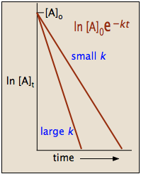
First-order:

$[A]_t = [A]_0\, e^{-kt}$

This is just the exponential form of the logarithmic equation above. Concentration decays exponentially. Radioactive decay follows first-order kinetics; for example, $^{14}\text{C}$ decay has $k = 1.21 \times 10^{-4}\;\text{yr}^{-1}$, so you can calculate how much remains in an archaeological sample after a given number of years.

Second-order:

$[A]_t = \frac{[A]_0}{1 + [A]_0\, kt}$

Here the concentration drops quickly at first, then tails off more slowly. The dimerization of cyclopentadiene in solution is a classic example. Because $k$ carries units of $\text{M}^{-1}\text{s}^{-1}$ for second-order reactions, the initial concentration directly affects how fast the reaction appears to proceed.

Calculating Half-Life

Half-Life Equations

The half-life ($t_{1/2}$) is the time required for $[A]$ to drop to $\frac{1}{2}[A]_0$. You derive each expression by substituting $[A]_t = \frac{[A]_0}{2}$ into the corresponding integrated rate law and solving for $t$.

First-order:

$t_{1/2} = \frac{\ln 2}{k}$

This depends only on $k$, not on $[A]_0$. That's the signature feature of first-order kinetics: every half-life is the same length, no matter how much reactant remains.

Second-order:

$t_{1/2} = \frac{1}{k[A]_0}$

Here the half-life is inversely proportional to the initial concentration. As the reaction proceeds and $[A]$ decreases, each successive half-life gets longer.

Zero-order:

$t_{1/2} = \frac{[A]_0}{2k}$

The half-life is directly proportional to $[A]_0$. Each successive half-life is shorter than the last because the concentration (and therefore the "new" $[A]_0$) keeps shrinking while the rate stays constant.

Half-Life Behavior by Order

How the half-life changes with concentration is itself a diagnostic tool:

• First-order (e.g., decomposition of $\text{N}_2\text{O}_5$): Measure half-lives at different starting concentrations. If they're all the same, the reaction is first-order.
• Second-order (e.g., dimerization reactions): Half-life gets longer as the reactant is consumed. Doubling $[A]_0$ cuts the half-life in half.
• Zero-order (e.g., enzyme-catalyzed reactions at substrate saturation): Half-life gets shorter as the reactant is consumed. Doubling $[A]_0$ doubles the half-life.

Reaction Order Analysis with Integrated Rate Laws

Graphical Analysis

The most reliable way to determine reaction order from experimental data is to make three plots and see which one gives a straight line.

1. Plot $[A]$ vs. $t$. If this is linear, the reaction is zero-order. The slope equals $-k$.
2. Plot $\ln[A]$ vs. $t$. If this is linear, the reaction is first-order. The slope equals $-k$.
3. Plot $\frac{1}{[A]}$ vs. $t$. If this is linear, the reaction is second-order. The slope equals $+k$.

Only one of these three plots will be linear (assuming the reaction cleanly follows a single order). The y-intercept in each case gives you the corresponding function of $[A]_0$ (i.e., $[A]_0$, $\ln[A]_0$, or $\frac{1}{[A]_0}$).

Confirming Reaction Order

Graphical analysis gives you the order, but it's good practice to confirm with half-life data. Run the reaction at two or more different initial concentrations and compare the measured half-lives:

• If $t_{1/2}$ stays constant across different $[A]_0$ values, the reaction is first-order.
• If $t_{1/2}$ is inversely proportional to $[A]_0$, the reaction is second-order.
• If $t_{1/2}$ is directly proportional to $[A]_0$, the reaction is zero-order.

As a concrete example, consider the gas-phase decomposition of $\text{N}_2\text{O}_5$. Plotting $\ln[\text{N}_2\text{O}_5]$ vs. time produces a straight line, while the other two plots curve. The measured half-life is approximately 22 minutes regardless of whether you start with 0.020 M or 0.010 M. Both observations confirm first-order kinetics, and the rate constant can be read directly from the slope of the linear plot: $k = 3.2 \times 10^{-2}\;\text{min}^{-1}$.