3.2 Second-Order Differential Equations

Second-order differential equations are a key part of solving complex real-world problems. They help us model things like springs, pendulums, and electrical circuits, giving us insights into how these systems behave over time.

These equations are more complex than first-order ones, but they're super useful. We'll learn how to classify them, solve different types, and apply them to practical situations. It's like unlocking a new toolbox for tackling tricky math problems.

Classifying Second-Order Linear Differential Equations

Identifying Second-Order Linear Differential Equations

• A second-order linear differential equation has the form $a(t)y''+b(t)y'+c(t)y=g(t)$
  • $a(t)$, $b(t)$, $c(t)$, and $g(t)$ are continuous functions of $t$
  • $a(t) \neq 0$ for the equation to be second-order
• Examples of second-order linear differential equations:
  • $y''+4y'+3y=e^{-t}$
  • $t^2y''+ty'+y=\sin(t)$

Homogeneous and Nonhomogeneous Equations

• A second-order linear differential equation is homogeneous if $g(t)=0$
  • Example: $y''+4y'+3y=0$
• A second-order linear differential equation is nonhomogeneous if $g(t) \neq 0$
  • Example: $y''+4y'+3y=e^{-t}$

Constant-Coefficient and Variable-Coefficient Equations

• The coefficients $a(t)$, $b(t)$, and $c(t)$ can be constant or variable
  • Constant-coefficient equations have coefficients that are constants ($a$, $b$, $c$)
    • Example: $y''+4y'+3y=e^{-t}$
  • Variable-coefficient equations have coefficients that are functions of $t$
    • Example: $t^2y''+ty'+y=\sin(t)$

Standard Form of Second-Order Linear Differential Equations

• A second-order linear differential equation is in standard form when $a(t)=1$
  • Example: $y''+4y'+3y=e^{-t}$ is in standard form
  • If $a(t) \neq 1$, divide the equation by $a(t)$ to obtain standard form

Solving Homogeneous Second-Order Linear Equations

General Solution of Homogeneous Equations

• The general solution of a homogeneous second-order linear differential equation with constant coefficients is $y=c_1y_1+c_2y_2$
  • $y_1$ and $y_2$ are linearly independent solutions
  • $c_1$ and $c_2$ are arbitrary constants
• The characteristic equation of $ay''+by'+cy=0$ is $ar^2+br+c=0$
  • The roots of the characteristic equation determine the form of the general solution

Real and Distinct Roots

• If the roots ($r_1$, $r_2$) of the characteristic equation are real and distinct, the general solution is $y=c_1e^{r_1t}+c_2e^{r_2t}$
• Example: For $y''-5y'+6y=0$, the characteristic equation is $r^2-5r+6=0$
  • The roots are $r_1=2$ and $r_2=3$
  • The general solution is $y=c_1e^{2t}+c_2e^{3t}$

Real and Repeated Roots

• If the roots of the characteristic equation are real and repeated ($r$), the general solution is $y=(c_1+c_2t)e^{rt}$
• Example: For $y''-6y'+9y=0$, the characteristic equation is $r^2-6r+9=0$
  • The repeated root is $r=3$
  • The general solution is $y=(c_1+c_2t)e^{3t}$

Complex Conjugate Roots

• If the roots of the characteristic equation are complex conjugates ($\alpha \pm i\beta$), the general solution is $y=e^{\alpha t}(c_1\cos \beta t+c_2\sin \beta t)$
• Example: For $y''+4y'+5y=0$, the characteristic equation is $r^2+4r+5=0$
  • The complex conjugate roots are $-2 \pm i$
  • The general solution is $y=e^{-2t}(c_1\cos t+c_2\sin t)$

Wronskian and Linear Independence

• The Wronskian can determine if two solutions are linearly independent
  • For solutions $y_1$ and $y_2$, the Wronskian is $W(y_1,y_2)=y_1y_2'-y_1'y_2$
  • If $W(y_1,y_2) \neq 0$ for some $t$, then $y_1$ and $y_2$ are linearly independent

Finding Particular Solutions of Nonhomogeneous Equations

General Solution of Nonhomogeneous Equations

• The general solution of a nonhomogeneous second-order linear differential equation is the sum of:
  • The general solution of the corresponding homogeneous equation (complementary solution)
  • A particular solution of the nonhomogeneous equation
• Example: For $y''+4y'+3y=e^{-t}$, the general solution is $y=c_1y_1+c_2y_2+y_p$
  • $c_1y_1+c_2y_2$ is the complementary solution
  • $y_p$ is a particular solution

Method of Undetermined Coefficients

• The method of undetermined coefficients finds a particular solution when $g(t)$ is a polynomial, exponential, sine, cosine, or a combination of these functions
• Assume a particular solution with unknown coefficients based on the form of $g(t)$
  • Example: For $y''+4y'+3y=e^{-t}$, assume $y_p=Ae^{-t}$
• Substitute the assumed solution into the differential equation and solve for the unknown coefficients
  • For $y''+4y'+3y=e^{-t}$, substituting $y_p=Ae^{-t}$ yields $A=\frac{1}{2}$
  • The particular solution is $y_p=\frac{1}{2}e^{-t}$

Method of Variation of Parameters

• The method of variation of parameters finds a particular solution for any continuous $g(t)$
• Let $y_1$ and $y_2$ be linearly independent solutions of the corresponding homogeneous equation
• A particular solution is given by $y_p=u_1y_1+u_2y_2$, where:
  • $u_1=-\int \frac{y_2g(t)}{W(y_1,y_2)}dt$
  • $u_2=\int \frac{y_1g(t)}{W(y_1,y_2)}dt$
  • $W(y_1,y_2)$ is the Wronskian of $y_1$ and $y_2$

Superposition Principle

• The superposition principle states that if:
  • $y_1$ is a solution to $a(t)y''+b(t)y'+c(t)y=g_1(t)$
  • $y_2$ is a solution to $a(t)y''+b(t)y'+c(t)y=g_2(t)$
• Then $y_1+y_2$ is a solution to $a(t)y''+b(t)y'+c(t)y=g_1(t)+g_2(t)$
• This principle allows for breaking down complex nonhomogeneous terms into simpler components

Applications of Second-Order Differential Equations

Modeling Simple Harmonic Motion

• Second-order differential equations can model simple harmonic motion
  • Examples include mass-spring systems and pendulums
  • The acceleration is proportional to the displacement
• The equation of motion for a simple harmonic oscillator is $my''+cy'+ky=F(t)$
  • $m$ is mass, $c$ is the damping coefficient, $k$ is the spring constant
  • $F(t)$ is the external force

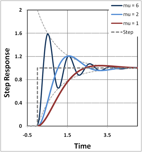
Characterizing Oscillator Behavior

• The natural frequency $\omega_n$ and the damping ratio $\zeta$ characterize the oscillator's behavior
  • $\omega_n=\sqrt{\frac{k}{m}}$ and $\zeta=\frac{c}{2\sqrt{mk}}$
• The system is underdamped if $0<\zeta<1$, critically damped if $\zeta=1$, and overdamped if $\zeta>1$
  • Underdamped systems exhibit oscillatory behavior with decreasing amplitude
  • Critically damped systems return to equilibrium as quickly as possible without oscillating
  • Overdamped systems return to equilibrium slowly without oscillating

Other Physical Applications

• Second-order differential equations can model various physical phenomena
  • Example: RLC circuits, where the current satisfies a second-order differential equation
• Resonance occurs when the external force frequency matches the system's natural frequency
  • This leads to large-amplitude oscillations
  • Example: A resonant frequency can cause a bridge to oscillate dangerously