3.2 Lagrange interpolation

Lagrange interpolation is a powerful technique for constructing polynomials that pass through given data points. It's a key method in approximating functions and fitting data, making it essential for various scientific and engineering applications.

The formula uses Lagrange basis polynomials to create a unique polynomial of degree ≤ n-1 for n data points. This method's versatility and mathematical foundations make it a cornerstone in computational mathematics and numerical analysis.

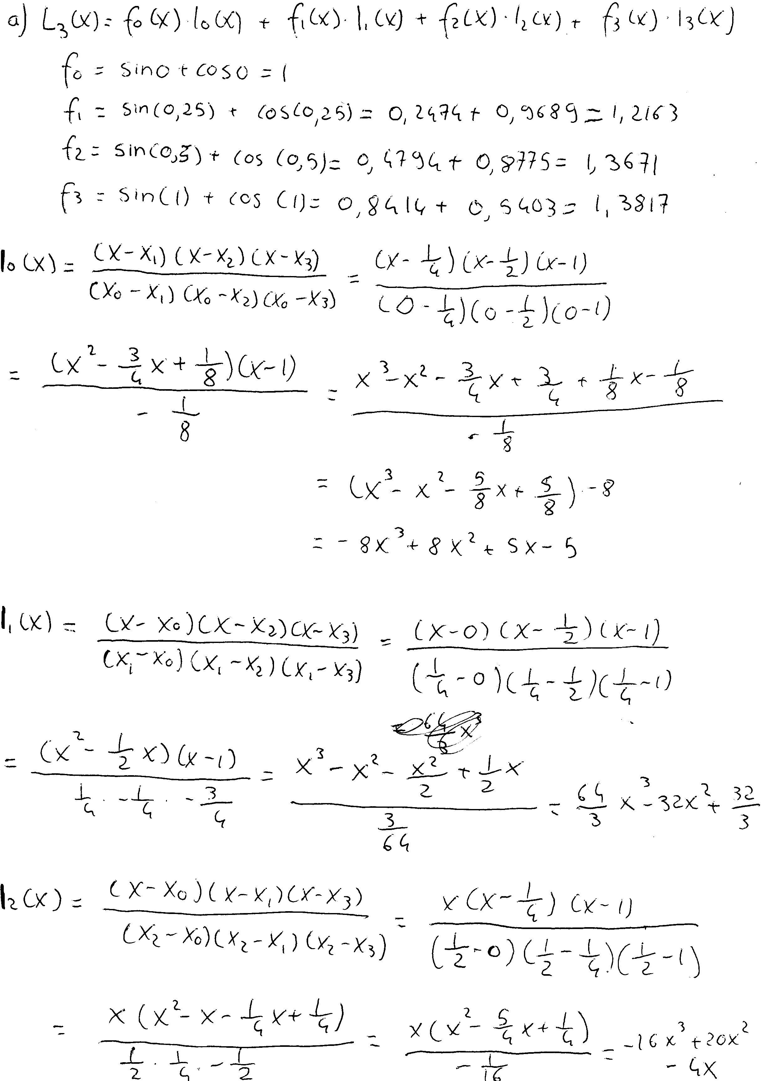
Lagrange Interpolation Formula

Polynomial Construction and Properties

• Lagrange interpolation constructs a unique polynomial of degree ≤ n-1 passing through n given data points
• Formula expressed as $P(x) = \sum_{i=1}^n y_i \cdot L_i(x)$, where yi are function values and Li(x) are Lagrange basis polynomials
• Resulting polynomial P(x) passes through all given data points (xi, yi)
• Uniqueness based on fundamental theorem of algebra and n-1 degree polynomial determined by n points
• Applications include function approximation, numerical integration, and data fitting in scientific and engineering fields (computational fluid dynamics, signal processing)

Mathematical Foundations

• Lagrange basis polynomials Li(x) defined as $L_i(x) = \prod_{j \neq i} \frac{(x - x_j)}{(x_i - x_j)}$, where xi are given data points
• Each Li(x) has property Li(xj) = 1 if i = j, and Li(xj) = 0 if i ≠ j, ensuring interpolation
• Computation involves calculating product of linear terms (x - xj) / (xi - xj) for all j ≠ i
• Efficient algorithms often use nested multiplication and Horner's method for polynomial evaluation
• Numerical stability crucial, especially for large data sets or closely spaced points

Lagrange Basis Polynomials

Computation and Construction

• Fundamental building blocks of Lagrange interpolation formula, each corresponding to specific data point
• Computation involves product of linear terms for all j ≠ i
• Construction of interpolating polynomial requires computing all basis polynomials
• Weighted sum of basis polynomials formed using given function values
• Example: For data points (1, 2), (2, 3), (3, 5), basis polynomials are: $L_1(x) = \frac{(x-2)(x-3)}{(1-2)(1-3)}$ $L_2(x) = \frac{(x-1)(x-3)}{(2-1)(2-3)}$ $L_3(x) = \frac{(x-1)(x-2)}{(3-1)(3-2)}$

Properties and Applications

• Each Li(x) equals 1 at its corresponding point and 0 at others
• Sum of all basis polynomials equals 1 for any x value
• Used in numerical integration techniques (Gaussian quadrature)
• Basis for constructing other interpolation methods (Hermite interpolation)
• Can be generalized to multidimensional interpolation (tensor product Lagrange polynomials)

Error Bounds and Convergence of Lagrange Interpolation

Error Analysis

• Error formula: $f(x) - P(x) = \frac{f^{(n)}(\xi)}{n!} \cdot \prod_{i=1}^n (x - x_i)$, where ξ is in interval containing x and all xi
• Error bound depends on function smoothness and interpolation point distribution
• Runge's phenomenon shows oscillations and divergence near endpoints for equally spaced points (example: Runge function $f(x) = \frac{1}{1 + 25x^2}$ on [-1, 1])
• Lebesgue constant measures stability and affects convergence properties

Convergence Properties and Improvements

• Guaranteed convergence for continuous functions on closed interval using Chebyshev nodes
• Chebyshev nodes defined as $x_k = \cos\left(\frac{2k-1}{2n}\pi\right)$, k = 1, ..., n
• Adaptive node selection strategies improve convergence and stability (Chebyshev points, Leja points)
• Barycentric form of Lagrange interpolation enhances numerical stability
• Error can be reduced by increasing polynomial degree or using piecewise interpolation (splines)