Unconstrained optimization is all about finding the best solution without limits. It's like searching for the highest mountain peak or the deepest valley, but in math. This technique is super useful in , data analysis, and even training AI.

The key is to understand the problem's structure and choose the right method to solve it. Sometimes, you're looking for the absolute best answer, while other times, a good enough solution will do. It's all about balancing accuracy and speed.

Unconstrained Optimization

Definition and Applications

Top images from around the web for Definition and Applications
  • Unconstrained optimization finds the minimum or maximum of a function without restrictions on variables
  • denoted as f(x), where x represents a vector of decision variables
  • Used in machine learning, data fitting, and parameter estimation (neural network training, curve fitting)
  • Solved using analytical methods for simple functions or numerical methods for complex cases (, )
  • Aims to find the , but local optima may be relevant in certain scenarios (protein folding)
  • Computational efficiency and convergence speed guide algorithm selection (trade-off between accuracy and speed)

Computational Considerations

  • Global optimum discovery challenging for (multiple )
  • Local optima may suffice for certain applications (image processing, financial modeling)
  • Algorithm selection depends on problem characteristics (function smoothness, dimensionality)
  • Scalability crucial for high-dimensional problems (optimization in deep learning)
  • Parallel computing techniques enhance performance for large-scale optimization (distributed optimization)
  • Stochastic methods handle noisy or uncertain objective functions (reinforcement learning)

Formulating Unconstrained Problems
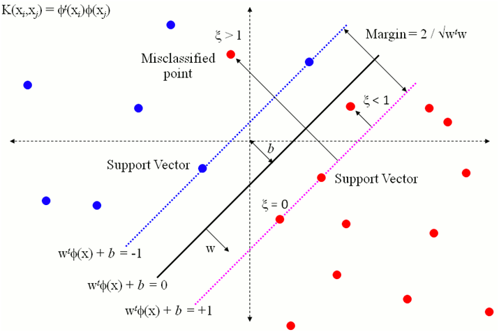
Problem Structure

  • Standard form min f(x) or max f(x), where f(x) represents the objective function
  • Key components objective function, decision variables, feasible region (entire function domain)
  • vector and H(x) crucial for analysis and solution
  • Domain of objective function defines search space for optimization algorithm
  • Proper scaling of variables and normalization impact algorithm performance
  • Initial starting point(s) selection important for iterative optimization methods

Problem Refinement

  • Objective function complexity affects solution approach (linear vs. nonlinear optimization)
  • techniques simplify high-dimensional problems (principal component analysis)
  • added to objective function to prevent overfitting (L1, L2 regularization)
  • handled through scalarization or Pareto optimization
  • assesses impact of parameter variations on optimal solution
  • accounts for uncertainties in problem formulation (min-max optimization)

Convexity of Objective Functions
Convexity Properties

  • guarantees unique global minimum for unconstrained problems
  • Function f(x) convex if line segment between any two points on graph lies above or on graph
  • Second-order condition for convexity Hessian matrix H(x) positive semidefinite for all x in domain
  • Convex functions local minimum also global minimum, simplifying optimization
  • Non-convex functions may have multiple local minima, requiring global optimization techniques
  • approximates non-convex problems with convex ones for easier solving

Implications for Optimization

  • Convexity ensures gradient-based methods converge to global optimum (gradient descent)
  • Efficient algorithms exist for convex optimization (interior point methods)
  • Convex problems solved in polynomial time, unlike general non-convex problems
  • Duality theory applies to convex problems, providing powerful analysis tools
  • Convex optimization problems have unique solutions, ensuring consistency
  • Decomposition methods effective for large-scale convex problems (primal-dual decomposition)

Optimality Conditions for Unconstrained Problems

First-Order Conditions

  • gradient ∇f(x*) = 0 at optimal point x*
  • (∇f(x) = 0) crucial for identifying potential optimal solutions
  • Include local minima, maxima, and saddle points
  • Karush- (KKT) conditions reduce to first-order necessary condition for unconstrained problems
  • Gradient-based methods use first-order information to iteratively approach optimal solution
  • follows negative gradient direction

Second-Order Conditions

  • Hessian matrix H(x*) positive semidefinite at optimal point x*
  • for local minimum Hessian matrix H(x*) positive definite at critical point x*
  • Newton's method and quasi-Newton methods utilize second-order information
  • ideal for second-order methods, faster than first-order methods
  • combines first and second-order information efficiently
  • use second-order information to define local quadratic models

Key Terms to Review (34)

∇f(x): The symbol ∇f(x) represents the gradient of a scalar function f at point x, indicating the direction and rate of fastest increase of the function. It is a vector field that contains all of the partial derivatives of f with respect to its variables, providing crucial information for optimization techniques and identifying local extrema.
Conjugate Gradient Method: The conjugate gradient method is an efficient algorithm for solving large systems of linear equations, particularly those that are symmetric and positive definite. This method is iterative, which means it approaches the solution gradually, making it especially suitable for problems where the matrix involved is sparse. By combining gradient descent techniques with the concept of conjugate directions, this method can achieve convergence faster than traditional methods, making it a favorite in numerical analysis.
Convergence Rate: The convergence rate refers to the speed at which a sequence or iterative method approaches its limit or desired solution. In numerical methods, this concept is crucial because it helps determine how quickly algorithms can produce accurate results, impacting efficiency and resource usage in computations.
Convex Relaxation: Convex relaxation is a technique used in optimization to transform a complex, non-convex problem into a simpler convex problem, making it easier to solve. This process often involves approximating the original problem by relaxing some of its constraints or altering the objective function, allowing for the application of efficient convex optimization algorithms. By finding a solution to the relaxed problem, insights or bounds on the solution to the original problem can be derived, which is especially useful in fields like machine learning and operations research.
Convexity: Convexity refers to the property of a set or function where, for any two points within that set or on the graph of that function, the line segment connecting them lies entirely within the set or above the graph. This concept is crucial in optimization since convex functions have unique global minima, making them easier to analyze and solve. Understanding convexity helps in recognizing when optimization problems can be efficiently tackled using specific algorithms, leading to more effective solutions.
Dimensionality reduction: Dimensionality reduction is a technique used to reduce the number of input variables in a dataset while preserving its essential features. This process helps in simplifying models, improving computational efficiency, and aiding visualization, making it easier to analyze data without significant loss of information. It is especially important when dealing with high-dimensional data that can lead to issues such as overfitting and increased computational costs.
F(x) ≥ 0: The expression f(x) ≥ 0 indicates that the function f evaluated at x is non-negative, meaning that the output of the function is either zero or positive. This condition is crucial in optimization problems as it helps define feasible regions where solutions can exist, ensuring that certain constraints are met in real-world applications.
First-order necessary condition: The first-order necessary condition is a mathematical criterion used to determine the optimality of a function, stating that at any local extremum, the first derivative of the function must equal zero. This condition helps identify potential maximum and minimum points in unconstrained optimization problems, indicating where the slope of the tangent line is horizontal. Understanding this concept is essential for finding optimal solutions in various optimization tasks.
Global optimum: A global optimum refers to the best possible solution across the entire feasible region of an optimization problem, where the objective function achieves its minimum or maximum value. This concept is crucial in understanding how optimization problems are solved, particularly in the context of unconstrained optimization where no limits restrict the variable values. Identifying a global optimum ensures that the most efficient outcome is achieved rather than settling for a local optimum, which may only represent a best solution within a limited range.
Gradient: The gradient is a vector that represents the direction and rate of the steepest ascent of a function. In the context of optimization, it plays a crucial role as it indicates how to adjust the variables to find the minimum or maximum values of a function. Understanding the gradient allows for efficient navigation through multidimensional spaces, guiding optimization algorithms toward optimal solutions.
Gradient Descent: Gradient descent is an optimization algorithm used to minimize a function by iteratively moving towards the steepest descent, as defined by the negative of the gradient. This method is fundamental in various mathematical and computational applications, facilitating solutions to problems such as fitting models to data or finding optimal parameters for algorithms. By adjusting parameters based on the slope of the function, gradient descent allows for effective convergence toward minima in both linear and nonlinear contexts.
Hessian matrix: The Hessian matrix is a square matrix of second-order partial derivatives of a scalar-valued function, providing crucial information about the curvature of the function's surface. It is used primarily in optimization problems to assess the local behavior of functions near critical points, helping to determine whether these points are minima, maxima, or saddle points. Understanding the Hessian is essential for techniques that rely on second derivative information, particularly when finding optimal solutions in both constrained and unconstrained scenarios.
Karush-Kuhn-Tucker Conditions: The Karush-Kuhn-Tucker (KKT) conditions are a set of mathematical conditions used to determine the optimal solutions of constrained optimization problems. These conditions extend the method of Lagrange multipliers, providing necessary conditions for a solution to be optimal when there are inequality constraints involved. The KKT conditions are critical in formulating and solving problems that involve maximizing or minimizing objective functions subject to constraints.
Kuhn-Tucker: The Kuhn-Tucker conditions are a set of mathematical conditions used to solve optimization problems that involve constraints, particularly in the context of non-linear programming. They extend the method of Lagrange multipliers by incorporating inequality constraints, providing necessary conditions for a solution to be optimal when certain criteria are met. These conditions help identify local maxima and minima in functions with constraints, allowing for a deeper understanding of optimization in various fields.
Lagrange: Lagrange refers to Joseph-Louis Lagrange, a prominent mathematician known for his contributions to optimization, particularly in the method of Lagrange multipliers. This method is crucial for solving constrained optimization problems, allowing one to find the local maxima and minima of a function subject to equality constraints. The connection to optimization extends into various fields, including economics, engineering, and physics, where it helps in determining optimal solutions under given conditions.
Local minima: Local minima are points in a function where the value of the function is lower than the values at nearby points, indicating that the function has reached a local low point in its vicinity. These points play a critical role in optimization problems, as they can represent solutions that minimize a given objective function, and finding them is essential for understanding the behavior of functions in various contexts.
Machine Learning: Machine learning is a branch of artificial intelligence that focuses on the development of algorithms and statistical models that enable computers to perform tasks without explicit instructions, relying instead on patterns and inference from data. It plays a crucial role in analyzing large datasets, optimizing processes, and making predictions, which are foundational aspects in various computational fields.
Multi-objective optimization: Multi-objective optimization is the process of optimizing two or more conflicting objectives simultaneously, often requiring trade-offs among them. This approach recognizes that many real-world problems involve multiple criteria that must be balanced, leading to a set of optimal solutions known as Pareto optimal solutions. It is particularly relevant when there are competing goals, such as maximizing profit while minimizing environmental impact.
Newton's Method: Newton's Method is an iterative numerical technique used to find approximate solutions to equations, particularly useful for locating roots of functions. This method leverages the concept of linear approximation, using the derivative to refine guesses and converge on a solution rapidly. It connects closely with various computational approaches, including fixed-point iteration, optimization problems, and even applications in finance and machine learning.
Non-convex functions: Non-convex functions are mathematical functions where the line segment connecting any two points on the graph does not lie entirely above the graph itself. This characteristic often results in multiple local minima and maxima, making optimization challenges more complex. Non-convex functions play a crucial role in unconstrained optimization because they can lead to difficulties in finding the global optimum due to the presence of numerous peaks and valleys.
Objective Function: An objective function is a mathematical expression that defines the goal of an optimization problem, typically representing a quantity that needs to be maximized or minimized. In various contexts, this function serves as the basis for determining the best solution among feasible options, guiding decisions based on certain criteria. Understanding how to formulate and manipulate the objective function is crucial for effectively applying optimization techniques across different scenarios.
Optimality conditions: Optimality conditions are criteria that help identify the best solution or point in an optimization problem, ensuring that it is either a maximum or minimum value. These conditions are crucial for determining when a function's gradient is zero, indicating that a local extremum may be present, and they guide the search for optimal solutions in unconstrained optimization problems.
Quadratic convergence: Quadratic convergence refers to a specific rate at which a sequence converges to a limit, where the error term is squared at each iteration. This means that if a method exhibits quadratic convergence, the number of correct digits approximately doubles with each iteration, leading to extremely rapid convergence to the solution. This property is particularly significant in numerical methods, optimization techniques, and algorithms used in machine learning, as it greatly enhances efficiency and reduces computational time.
Regularization Terms: Regularization terms are additional components added to an optimization problem to prevent overfitting by penalizing complex models. They act as constraints that modify the objective function, ensuring that the learned model remains simple and generalizes well to unseen data. Regularization helps balance the trade-off between fitting the training data closely and maintaining model simplicity.
Resource allocation: Resource allocation refers to the process of distributing available resources in an optimal manner to achieve specific goals or objectives. This process is crucial in decision-making where limited resources must be assigned efficiently among competing activities, impacting various areas such as production, budget management, and project planning.
Robust Optimization: Robust optimization is a method in optimization that focuses on finding solutions that remain effective under uncertainty and variability in data. This approach aims to produce solutions that are less sensitive to fluctuations, ensuring that performance remains acceptable even when the conditions deviate from expectations. By incorporating uncertainty directly into the optimization process, robust optimization enhances the reliability of solutions compared to traditional methods.
Saddle Point: A saddle point is a point on the surface of a function where the slope is zero in all directions, meaning it is neither a local maximum nor a local minimum. It can be visualized as a point that looks like a saddle, with some directions curving upwards and others curving downwards. This unique characteristic makes saddle points significant in optimization, particularly in understanding the behavior of functions in unconstrained optimization problems.
Second-order necessary condition: The second-order necessary condition is a criterion used in optimization to determine whether a point is a local minimum. Specifically, for a function to have a local minimum at a certain point, the first derivative must be zero, and the second derivative must be non-negative. This condition is crucial in understanding the nature of critical points in unconstrained optimization.
Second-order sufficient condition: The second-order sufficient condition is a criterion used in optimization to determine whether a point is a local minimum or maximum based on the behavior of the function's second derivative. This condition specifically states that for a critical point to be a local minimum, the first derivative must equal zero and the second derivative must be positive, indicating that the function curves upward at that point. Conversely, for a local maximum, the second derivative should be negative, indicating that the function curves downward.
Sensitivity analysis: Sensitivity analysis is a technique used to determine how different values of an independent variable will impact a particular dependent variable under a given set of assumptions. This approach helps in understanding the influence of variations in input parameters on outcomes, which is crucial for making informed decisions in various mathematical and optimization models.
Stationary points: Stationary points are points on a function where the first derivative is zero or undefined, indicating potential locations for local maxima, minima, or saddle points. They are crucial in optimization as they help identify where a function may change direction, ultimately guiding the search for optimal values in a given problem.
Steepest descent method: The steepest descent method is an iterative optimization algorithm used to find the minimum of a function by moving in the direction of the steepest decrease of the function's value. This method uses the gradient of the function to determine the direction to move, which ensures that each step taken brings you closer to the minimum point. It's particularly useful in unconstrained optimization problems where no restrictions are placed on the variable values.
Stopping criteria: Stopping criteria are specific conditions or rules that determine when an optimization algorithm should cease its iterative process. These criteria are essential in unconstrained optimization, as they help ensure that the solution is sufficiently accurate or optimal while avoiding unnecessary computations. Establishing effective stopping criteria is crucial for balancing solution quality with computational efficiency.
Trust Region Methods: Trust region methods are optimization techniques that create a restricted area around the current point in the search space where a model is trusted to approximate the objective function accurately. These methods balance local and global search by adjusting the size of the trust region based on how well the model predicts the behavior of the objective function, making them particularly useful in solving nonlinear optimization problems, nonlinear systems of equations, and when implementing methods like Broyden's for updating Jacobians.
© 2024 Fiveable Inc. All rights reserved.
AP® and SAT® are trademarks registered by the College Board, which is not affiliated with, and does not endorse this website.