3.1 Expected value

Expected value is a fundamental concept in probability theory and statistics, quantifying the average outcome of a random variable. It serves as a measure of central tendency for probability distributions, enabling predictions and comparisons across various statistical applications.

Calculating expected value involves probability-weighted averages for discrete cases and integration for continuous cases. Understanding its properties, such as linearity and non-negativity, is crucial for deriving statistical theorems and conducting advanced analyses in theoretical statistics.

Definition of expected value

• Expected value forms a fundamental concept in probability theory and statistics, quantifying the average outcome of a random variable
• In theoretical statistics, expected value provides a measure of central tendency for probability distributions, enabling predictions and comparisons
• Serves as a crucial tool for analyzing and interpreting data in various statistical applications

Probability-weighted average

• Calculates the sum of all possible values multiplied by their respective probabilities
• Represents the long-term average outcome if an experiment is repeated infinitely
• Denoted mathematically as $E[X] = \sum_{i=1}^{n} x_i \cdot p(x_i)$ for discrete random variables
• Accounts for both the magnitude of outcomes and their likelihood of occurrence

Discrete vs continuous cases

• Discrete case involves summing over finite or countably infinite set of possible values
• Continuous case requires integration over the entire range of the random variable
• Continuous expected value expressed as $E[X] = \int_{-\infty}^{\infty} x \cdot f(x) dx$ where f(x) is the probability density function
• Transition from discrete to continuous involves replacing summation with integration and probability mass function with probability density function

Properties of expected value

• Expected value exhibits several key properties that make it a powerful tool in theoretical statistics
• These properties allow for manipulation and analysis of complex probabilistic scenarios
• Understanding these properties is crucial for deriving statistical theorems and conducting advanced analyses

Linearity of expectation

• States that the expected value of a sum equals the sum of individual expected values
• Expressed mathematically as $E[aX + bY] = aE[X] + bE[Y]$ for constants a and b and random variables X and Y
• Holds true even when random variables are dependent, making it a powerful tool in probability calculations
• Allows for simplification of complex problems by breaking them down into simpler components

Expected value of constants

• Expected value of a constant is the constant itself: $E[c] = c$ for any constant c
• Implies that adding or subtracting a constant from a random variable shifts its expected value by that amount
• Useful in standardizing random variables and transforming probability distributions
• Helps in understanding the impact of deterministic components in probabilistic models

Non-negativity

• Expected value of a non-negative random variable is always non-negative
• If X ≥ 0, then $E[X] ≥ 0$
• Extends to absolute values: $E[|X|] ≥ |E[X]|$
• Provides bounds and constraints in probability inequalities and statistical estimations

Calculation methods

• Various techniques exist for calculating expected values, depending on the nature of the random variable
• Selection of appropriate method is crucial for accurate results and efficient computation
• Understanding these methods is essential for applying expected value concepts to real-world problems

Discrete random variables

• Utilizes probability mass function (PMF) to compute expected value
• Involves summing the product of each possible value and its probability
• Formula: $E[X] = \sum_{x} x \cdot P(X = x)$ where x ranges over all possible values of X
• Applicable to finite and countably infinite sample spaces (coin flips, dice rolls)

Continuous random variables

• Employs probability density function (PDF) to calculate expected value
• Requires integration over the entire range of the random variable
• Formula: $E[X] = \int_{-\infty}^{\infty} x \cdot f(x) dx$ where f(x) is the PDF of X
• Used for variables with uncountably infinite possible values (time intervals, measurements)

Using probability distributions

• Leverages known properties of standard probability distributions to compute expected values
• Involves identifying the distribution type and its parameters
• Utilizes pre-derived formulas for expected values of common distributions (normal, exponential, Poisson)
• Simplifies calculations for well-studied probability models in theoretical statistics

Conditional expected value

• Extends the concept of expected value to scenarios where additional information is available
• Plays a crucial role in Bayesian statistics and decision theory
• Allows for more precise predictions by incorporating relevant contextual information

Definition and interpretation

• Represents the expected value of a random variable given that another event has occurred
• Denoted as $E[X|Y]$ for random variables X and Y
• Calculated using the conditional probability distribution of X given Y
• Provides a way to update expectations based on new information or observations

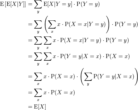
Law of total expectation

• Also known as the law of iterated expectation or tower property
• States that $E[X] = E[E[X|Y]]$ for random variables X and Y
• Allows decomposition of expected value calculations into conditional components
• Useful in solving complex probability problems and deriving statistical theorems
• Applications in decision trees, Markov chains, and hierarchical models

Applications in statistics

• Expected value concepts find widespread use across various domains of statistical analysis
• Serve as foundational tools for developing statistical models and making inferences
• Enable quantitative decision-making in uncertain environments

Mean of probability distributions

• Expected value represents the theoretical mean or average of a probability distribution
• Provides a measure of central tendency for symmetric and asymmetric distributions
• Used to characterize and compare different probability models
• Essential in hypothesis testing and parameter estimation (sample mean as estimator of population mean)

Risk assessment and decision theory

• Utilizes expected value to quantify potential outcomes in uncertain scenarios
• Helps in evaluating and comparing different strategies or decisions
• Applied in fields like insurance, finance, and project management
• Incorporates utility functions to account for risk preferences in decision-making processes

Financial modeling

• Expected value concepts crucial in pricing financial instruments (options, futures)
• Used in portfolio theory to optimize risk-return tradeoffs
• Employed in calculating present and future values of cash flows
• Fundamental in assessing investment strategies and conducting risk analysis

Variance and expected value

• Variance and expected value are closely related concepts in probability theory
• Together, they provide a comprehensive description of a random variable's distribution
• Understanding their relationship is crucial for advanced statistical analyses

Relationship between variance and expectation

• Variance measures the spread or dispersion of a random variable around its expected value
• Defined as the expected value of the squared deviation from the mean: $Var(X) = E[(X - E[X])^2]$
• Alternative formula: $Var(X) = E[X^2] - (E[X])^2$
• Variance is always non-negative, equaling zero only for constants

Covariance and correlation

• Covariance extends the concept of variance to measure the joint variability of two random variables
• Defined as $Cov(X,Y) = E[(X - E[X])(Y - E[Y])]$
• Correlation normalizes covariance to provide a standardized measure of association
• Correlation coefficient: $\rho_{X,Y} = \frac{Cov(X,Y)}{\sqrt{Var(X)Var(Y)}}$
• Both concepts crucial in multivariate analysis, regression, and time series modeling

Moment-generating functions

• Powerful tool in theoretical statistics for analyzing probability distributions
• Encapsulates all moments of a distribution in a single function
• Facilitates derivation of distribution properties and proving theoretical results

Definition and properties

• Moment-generating function (MGF) of a random variable X defined as $M_X(t) = E[e^{tX}]$
• Exists only if the expectation is finite for t in some neighborhood of 0
• Uniquely determines the probability distribution if it exists
• Useful for proving convergence in distribution and deriving distribution of transformed random variables

Deriving expected value

• Expected value can be obtained by evaluating the first derivative of MGF at t = 0
• $E[X] = M'_X(0)$ where M'_X(t) denotes the derivative of MGF with respect to t
• Higher-order moments derived similarly: $E[X^n] = M^{(n)}_X(0)$ where M^(n)_X(t) is the nth derivative
• Provides an alternative method for calculating expected values and moments of distributions

Inequalities involving expected value

• Expected value inequalities provide bounds and constraints on probabilities and random variables
• Essential tools in theoretical statistics for proving theorems and deriving approximations
• Aid in understanding limitations and relationships between different probabilistic quantities

Markov's inequality

• Provides an upper bound on the probability that a non-negative random variable exceeds a certain value
• States that for a non-negative random variable X and a > 0, $P(X ≥ a) ≤ \frac{E[X]}{a}$
• Useful when only the expected value of a distribution is known
• Forms the basis for proving other probability inequalities (Chebyshev's inequality)

Jensen's inequality

• Applies to convex functions and expected values
• States that for a convex function f and random variable X, $f(E[X]) ≤ E[f(X)]$
• For concave functions, the inequality is reversed
• Has applications in information theory, optimization, and economic theory
• Used to derive bounds on expected values of transformed random variables

Expected value in specific distributions

• Understanding expected values of common probability distributions is crucial in theoretical statistics
• Provides insights into the behavior and properties of these distributions
• Facilitates modeling and analysis of various real-world phenomena

Bernoulli and binomial distributions

• Bernoulli distribution: $E[X] = p$ where p is the probability of success
• Binomial distribution: $E[X] = np$ where n is the number of trials
• Models discrete events with two possible outcomes (success/failure, yes/no)
• Applications in quality control, epidemiology, and survey sampling

Poisson distribution

• Expected value equals the rate parameter: $E[X] = \lambda$
• Models rare events occurring in a fixed interval of time or space
• Variance also equals λ, a unique property of the Poisson distribution
• Used in queueing theory, reliability analysis, and modeling count data

Normal distribution

• Expected value equals the location parameter μ: $E[X] = \mu$
• Symmetric distribution with bell-shaped curve
• Central to many statistical theories due to the Central Limit Theorem
• Widely used in natural and social sciences for modeling continuous variables

Estimation of expected value

• Estimating expected values from sample data is a fundamental task in statistical inference
• Bridges the gap between theoretical concepts and practical applications of statistics
• Crucial for making inferences about population parameters based on limited data

Sample mean as estimator

• Sample mean (x̄) serves as an unbiased estimator of the population mean (μ)
• Calculated as $\bar{x} = \frac{1}{n}\sum_{i=1}^{n} x_i$ for a sample of size n
• Converges to the true expected value as sample size increases (law of large numbers)
• Forms the basis for many statistical procedures (hypothesis tests, confidence intervals)

Properties of estimators

• Unbiasedness: $E[\bar{X}] = \mu$ (sample mean is an unbiased estimator of population mean)
• Consistency: estimator converges in probability to the true parameter as sample size increases
• Efficiency: measures the variance of the estimator relative to the theoretical lower bound
• Robustness: ability of the estimator to perform well under departures from assumed conditions
• Trade-offs often exist between these properties, influencing choice of estimators in practice