4.4 Small-signal models and block diagrams

Small-Signal Models of Synchronous Machines

Small-signal models let you study how a synchronous machine responds to small perturbations around a steady-state operating point. Instead of wrestling with the full nonlinear swing and flux-linkage equations, you linearize them so that standard linear-systems tools (transfer functions, eigenvalue analysis, block diagrams) become available. This is the foundation for assessing whether oscillations will grow or decay after a minor disturbance, and for tuning controllers like power system stabilizers (PSSs) and automatic voltage regulators (AVRs).

Linearization of the Machine Equations

The synchronous machine is governed by nonlinear differential equations relating rotor angle $\delta$, rotor speed $\omega$, flux linkages $\psi$, voltages, and torques. To linearize:

1. Choose an operating point. Pick the steady-state values $\delta_0, \omega_0, \psi_0, V_0, T_0$ that satisfy the nonlinear equations.
2. Introduce incremental variables. Replace each variable with its steady-state value plus a small deviation: $\delta = \delta_0 + \Delta\delta$, $\omega = \omega_0 + \Delta\omega$, etc.
3. Apply a Taylor series expansion to every nonlinear term and drop all second-order and higher products of the $\Delta$ quantities. For example, a term like $\sin\delta$ becomes $\sin\delta_0 + (\cos\delta_0)\,\Delta\delta$.
4. Subtract the steady-state equations so that only the incremental (small-signal) equations remain.

The result is a set of linear differential equations in the incremental state variables ($\Delta\delta$, $\Delta\omega$, $\Delta\psi_d$, $\Delta\psi_q$, …) driven by incremental inputs ($\Delta V_f$, $\Delta T_m$). These equations are valid only for small deviations; large disturbances require the full nonlinear model.

Representation of the Linearized Equations

Once linearized, the equations can be cast in two equivalent forms:

• Transfer functions describe single-input/single-output relationships in the Laplace (frequency) domain. For example, $\Delta\delta(s)/\Delta T_e(s)$ or $\Delta V_t(s)/\Delta V_f(s)$.
• State-space representations capture the full multi-input/multi-output dynamics in the time domain as a set of coupled first-order ODEs.

State-space form is generally preferred for multivariable analysis because it directly supports eigenvalue computation, controllability/observability tests, and state-feedback controller design.

Transfer Functions and State-Space Representations

Deriving Transfer Functions

1. Start from the linearized differential equations in the time domain.
2. Apply the Laplace transform to each equation, assuming zero initial conditions.
3. Algebraically solve for the desired output variable in terms of the desired input variable.

Common transfer functions you'll encounter:

• Rotor angle to electrical torque: $\Delta\delta(s)/\Delta T_e(s)$, which reveals the electromechanical oscillation mode.
• Rotor speed to mechanical torque: $\Delta\omega(s)/\Delta T_m(s)$, useful for governor tuning.
• Terminal voltage to field voltage: $\Delta V_t(s)/\Delta V_f(s)$, central to excitation-system design.

Each transfer function is a ratio of polynomials in $s$. The poles of that ratio are the natural modes of the subsystem, and their locations tell you whether the response is stable and well-damped.

State-Space Form

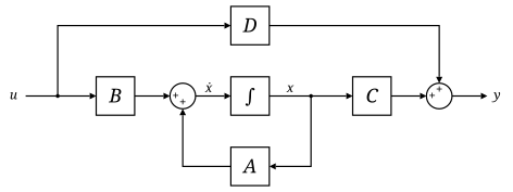
The full linearized model is written as:

$\dot{x} = Ax + Bu$

$y = Cx + Du$

where:

• $x$ is the state vector (e.g., $[\Delta\delta,\;\Delta\omega,\;\Delta\psi_d,\;\Delta\psi_q,\;\dots]^T$)
• $u$ is the input vector (e.g., $[\Delta T_m,\;\Delta V_f]^T$)
• $y$ is the output vector (e.g., $[\Delta V_t,\;\Delta P_e]^T$)
• $A$ is the state matrix, whose eigenvalues determine stability
• $B$, $C$, $D$ are the input, output, and feedthrough matrices

Why state-space matters:

• Stability is assessed directly from the eigenvalues of $A$.
• Controllability (can the inputs influence every mode?) and observability (can the outputs reveal every mode?) are checked with rank tests on $(A, B)$ and $(A, C)$.
• State-feedback and observer-based controllers can be designed systematically.

Block Diagrams for Synchronous Machines

Constructing Block Diagrams

Block diagrams translate the linearized equations into a visual signal-flow map. Each block represents a transfer function or gain, and arrows show how signals propagate.

1. Start with the mechanical subsystem. The classic swing equation in small-signal form gives a chain: $\Delta T_m - \Delta T_e \rightarrow \frac{1}{2Hs+D} \rightarrow \Delta\omega \rightarrow \frac{1}{s} \rightarrow \Delta\delta$, where $H$ is the inertia constant and $D$ is the damping coefficient.

2. Add the electrical subsystem. Connect $\Delta\delta$ and flux-linkage deviations back to the electrical torque $\Delta T_e$, creating a feedback path. The synchronizing torque coefficient $K_1$ and damping torque coefficient appear here.

3. Attach the excitation system. A block for the AVR and exciter links $\Delta V_t$ (or its error) to $\Delta V_f$, which in turn affects flux linkages and terminal voltage.

4. Include supplementary controllers. A PSS block typically feeds a stabilizing signal (derived from $\Delta\omega$ or $\Delta P_e$) into the excitation system to add damping torque.

5. Include the governor loop if mechanical power variations are of interest: the speed deviation $\Delta\omega$ feeds back through the governor and turbine transfer functions to produce $\Delta T_m$.

Feedback loops are the defining feature. The rotor angle feeds back through the electrical torque, the terminal voltage feeds back through the AVR, and speed feeds back through the governor. These loops are what make stability analysis non-trivial.

Interpreting and Simplifying Block Diagrams

• Identify the main loops. The electromechanical loop ($\Delta\delta \leftrightarrow \Delta T_e$) dominates low-frequency oscillations (typically 0.2–2 Hz). The excitation loop affects voltage regulation and can either help or hurt damping.
• Trace the effect of parameter changes. Increasing a gain (e.g., AVR gain) shifts pole locations; you can see which loop is affected by following the signal path.
• Apply block diagram algebra to reduce cascaded, parallel, and feedback blocks into simpler equivalent transfer functions. Standard reduction rules (e.g., Mason's gain formula) let you collapse the diagram to a single input-output transfer function when needed.

The visual layout makes it much easier to see where a new controller should inject its signal and which feedback path it modifies.

Stability and Dynamic Performance Analysis

Small-Signal Stability Assessment

Small-signal stability asks: after a tiny perturbation, do all state variables return to equilibrium, or does some oscillation grow?

The answer comes from the eigenvalues $\lambda_i = \sigma_i \pm j\omega_i$ of the state matrix $A$:

• If every eigenvalue has a negative real part ($\sigma_i < 0$), the system is stable and all modes decay.
• A positive real part on any eigenvalue means that mode is unstable and oscillations will grow.
• The imaginary part $\omega_i$ gives the oscillation frequency; the real part $\sigma_i$ determines the rate of decay or growth.
• The damping ratio of a complex eigenvalue pair is $\zeta = -\sigma / \sqrt{\sigma^2 + \omega^2}$. Low damping ratios (below ~0.05) flag poorly damped modes even if technically stable.

Participation factors, computed from the right and left eigenvectors, tell you which state variables are most involved in each mode. For instance, a participation factor analysis might reveal that a 1.2 Hz mode is dominated by $\Delta\delta$ and $\Delta\omega$ of a particular machine, pointing you to where a PSS would be most effective.

Graphical tools for stability assessment:

• Root locus plots show how eigenvalues migrate as a single parameter (e.g., AVR gain) varies.
• Bode and Nyquist plots of open-loop transfer functions give gain and phase margins for specific control loops.

Dynamic Performance Evaluation

Beyond just stable/unstable, you need to know how well the system responds:

• Time-domain simulations of the linearized model reveal settling time, overshoot, and oscillatory behavior after a step change in load or reference.
• Frequency-domain metrics such as bandwidth, gain margin, and phase margin quantify robustness to parameter uncertainty and unmodeled dynamics.
• Performance indices like damping ratio $\zeta$, settling time $t_s \approx 4/|\sigma|$, and rise time characterize the speed and quality of the response.

These analyses feed directly into controller design. If a particular electromechanical mode has poor damping, you design a PSS whose phase-lead characteristic adds positive damping torque at that mode's frequency. The small-signal model and block diagram let you verify the design analytically before running full nonlinear simulations.