3.1 Power flow problem formulation

Power Flow Problem Formulation

Power flow analysis determines the voltage magnitudes, voltage angles, and power flows at every bus in an electrical network under steady-state conditions. It's the foundational calculation engineers use to verify that a planned or operating power system can deliver power within acceptable voltage and loading limits. This topic covers how the problem is mathematically set up, how buses are classified, and how the nonlinear equations are solved iteratively.

Bus Admittance Matrix and Power Balance Equations

The power flow problem starts with a model of the network. The bus admittance matrix ($Y_{bus}$) captures the entire network topology and the admittances of every transmission line and transformer in a single square matrix, with dimensions $n \times n$ for an $n$-bus system.

Each diagonal element $Y_{ii}$ equals the sum of all admittances connected to bus $i$ (including shunt elements). Each off-diagonal element $Y_{ij}$ equals the negative of the admittance directly connecting bus $i$ to bus $j$. If buses $i$ and $j$ have no direct connection, $Y_{ij} = 0$, which is why $Y_{bus}$ is typically sparse for large systems.

Power balance equations are derived from Kirchhoff's Current Law (KCL). At each bus, the net injected power (generation minus load) must equal the total power flowing out through all connected lines. Written in terms of bus voltages and admittance elements:

$P_i = \sum_{j=1}^{n} |V_i||V_j||Y_{ij}| \cos(\theta_{ij} + \delta_j - \delta_i)$

$Q_i = -\sum_{j=1}^{n} |V_i||V_j||Y_{ij}| \sin(\theta_{ij} + \delta_j - \delta_i)$

where:

• $P_i$ and $Q_i$ are the net active and reactive power injections at bus $i$
• $|V_i|$ and $\delta_i$ are the voltage magnitude and angle at bus $i$
• $|Y_{ij}|$ and $\theta_{ij}$ are the magnitude and angle of the $(i,j)$ element of $Y_{bus}$

Note the sign convention on the reactive power equation: the negative sign appears because of how the sine term relates to reactive power consumption versus generation. Some textbooks fold this sign into the angle convention, so always check which form your course uses.

Complex Power Injections

The complex power injection at bus $i$ is:

$S_i = P_i + jQ_i = V_i I_i^*$

where $I_i^*$ is the complex conjugate of the net current injected at bus $i$. This net injection equals the sum of power flows from bus $i$ to every connected bus $j$:

$S_i = \sum_j S_{ij}$

The power flow on a single line from bus $i$ to bus $j$ is built up in three steps:

1. Express the line current using the admittance between the two buses: $I_{ij} = (V_i - V_j) Y_{ij}$

2. Form the complex power flow using the sending-end voltage and the conjugate of the line current: $S_{ij} = V_i \, I_{ij}^*= V_i (V_i - V_j)^* Y_{ij}^*$

3. Separate into real and imaginary parts to get the active power flow $P_{ij}$ and reactive power flow $Q_{ij}$ on that line.

This line-by-line formulation is what you use after solving the power flow to compute individual branch flows and losses.

Bus Classification in Power Systems

Every bus in the system is assigned one of three types, depending on which quantities are known (specified) and which must be solved for.

Slack Bus

The slack bus (also called the swing bus) serves as the voltage reference for the entire system. Its voltage magnitude and angle are both fixed, typically set to $1.0 \angle 0°$ in per-unit. Because total system losses aren't known until after the solution converges, the slack bus absorbs whatever active and reactive power mismatch remains. There is exactly one slack bus per system.

PV Bus

A PV bus (generator bus) has its active power injection $P$ and voltage magnitude $|V|$ specified. The unknowns to solve for are the voltage angle $\delta$ and the reactive power output $Q$. Any bus with a voltage-regulating generator is modeled this way. In practice, the generator's reactive output must stay within its capability limits; if $Q$ hits a limit during the iterative solution, the bus is temporarily converted to a PQ bus at that limit.

PQ Bus

A PQ bus (load bus) has both its active and reactive power injections $P$ and $Q$ specified. The unknowns are the voltage magnitude $|V|$ and angle $\delta$. Most buses in a real power system are PQ buses, representing loads such as residential areas, industrial facilities, or any bus without active voltage regulation.

Jacobian Matrix for Power Flow

Why an Iterative Method Is Needed

The power balance equations are nonlinear (they involve products of voltage magnitudes and trigonometric functions of angle differences). There's no closed-form solution, so you solve them iteratively. The Newton-Raphson method is the standard approach because of its fast (quadratic) convergence.

Jacobian Matrix Structure

At each iteration, Newton-Raphson linearizes the power balance equations around the current estimate. The linearized system is:

$\begin{bmatrix} \Delta P \\ \Delta Q \end{bmatrix} = \begin{bmatrix} J_1 & J_2 \\ J_3 & J_4 \end{bmatrix} \begin{bmatrix} \Delta \delta \\ \Delta |V| \end{bmatrix}$

The four submatrices of the Jacobian matrix $J$ are:

• $J_1 = \partial P / \partial \delta$ — sensitivity of active power to voltage angle changes
• $J_2 = \partial P / \partial |V|$ — sensitivity of active power to voltage magnitude changes
• $J_3 = \partial Q / \partial \delta$ — sensitivity of reactive power to voltage angle changes
• $J_4 = \partial Q / \partial |V|$ — sensitivity of reactive power to voltage magnitude changes

Each element is obtained by partially differentiating the power balance equations with respect to the corresponding unknown. The Jacobian must be recalculated (or updated) at every iteration because the operating point changes.

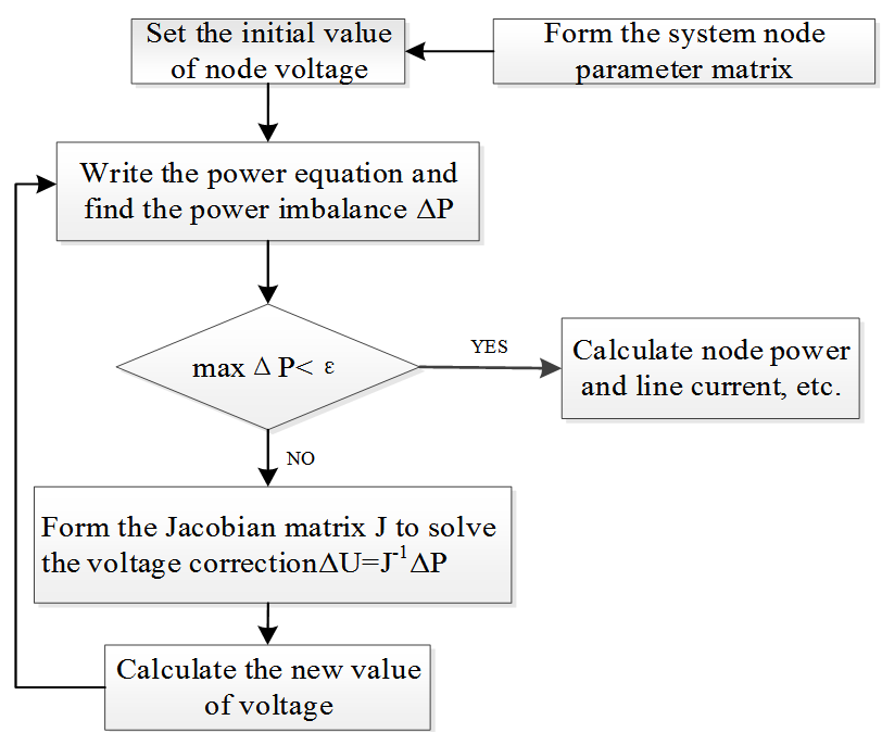
Newton-Raphson Solution Steps

1. Initialize all unknown voltages. A common starting point (flat start) is $|V| = 1.0$ p.u. and $\delta = 0°$ for every unknown bus.
2. Compute power mismatches $\Delta P_i$ and $\Delta Q_i$ at each bus by substituting current voltage estimates into the power balance equations and comparing with the specified values.
3. Check convergence. If all mismatches are below the tolerance (typically $10^{-3}$ p.u. or smaller), stop. The current voltages are the solution.
4. Build the Jacobian matrix $J$ using the current voltage estimates.
5. Solve the linear system for the correction vector: $\Delta X = J^{-1} \Delta F$ where $\Delta X = [\Delta \delta \; \Delta |V|]^T$ and $\Delta F = [\Delta P \; \Delta Q]^T$. In practice, you solve $J \, \Delta X = \Delta F$ using LU factorization rather than explicitly inverting $J$.
6. Update the unknowns: $X_{new} = X_{old} + \Delta X$
7. Return to Step 2 and repeat until convergence.

Most well-conditioned systems converge in 3–5 iterations with Newton-Raphson. If the system is heavily loaded or near a voltage collapse point, convergence may be slow or may fail entirely, which itself is a useful diagnostic indicator of system stress.