7.4 Step Functions and Discontinuous Forcing Functions

Step functions and discontinuous forcing functions are game-changers in differential equations. They let us model sudden changes, like flipping a switch or applying a force out of nowhere. It's like adding a plot twist to our math story!

Laplace transforms make dealing with these jumpy functions a breeze. We can turn tricky discontinuous problems into smooth algebraic ones. It's like having a secret weapon for solving real-world problems with sudden changes.

Step Functions

Heaviside Step Function and Unit Step Function

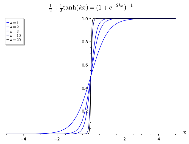
• Heaviside step function $H(t)$ represents a discontinuous function that jumps from 0 to 1 at $t=0$
  • Defined as $H(t) = 0$ for $t < 0$ and $H(t) = 1$ for $t \geq 0$
  • Useful for modeling sudden changes or switches in a system (turning on a light switch)
• Unit step function $u(t)$ is a shifted version of the Heaviside step function
  • Defined as $u(t) = 0$ for $t < 0$ and $u(t) = 1$ for $t \geq 0$
  • Can be expressed in terms of the Heaviside step function: $u(t) = H(t)$
  • Represents a unit change in a system at a specific time (applying a constant force at a given moment)

Piecewise Continuous Functions and Laplace Transforms

• Piecewise continuous functions are functions that are continuous on a finite number of intervals but may have discontinuities at the endpoints of these intervals
  • Can be represented using step functions (Heaviside or unit step) to define different pieces of the function
  • Example: $f(t) = \begin{cases} 0, & t < 0 \\ t, & 0 \leq t < 1 \\ 1, & t \geq 1 \end{cases}$ can be written as $f(t) = t[u(t) - u(t-1)] + u(t-1)$
• Laplace transform of step functions allows for solving differential equations with discontinuous forcing functions
  • Laplace transform of the Heaviside step function: $\mathcal{L}\{H(t)\} = \frac{1}{s}$
  • Laplace transform of the unit step function: $\mathcal{L}\{u(t)\} = \frac{1}{s}$
  • Laplace transform of a shifted unit step function: $\mathcal{L}\{u(t-a)\} = \frac{e^{-as}}{s}$, where $a$ is the shift amount

Discontinuous Forcing Functions

Discontinuous Forcing Functions and Dirac Delta Function

• Discontinuous forcing functions are functions that have sudden changes or jumps in their values
  • Can be represented using step functions (Heaviside or unit step) or the Dirac delta function
  • Example: a sudden impact force on a spring-mass system can be modeled using a step function or Dirac delta function
• Dirac delta function $\delta(t)$ is a generalized function that represents an infinitely high, infinitely narrow spike at $t=0$
  • Defined by its integral properties: $\int_{-\infty}^{\infty} \delta(t) dt = 1$ and $\int_{-\infty}^{\infty} f(t) \delta(t-a) dt = f(a)$
  • Useful for modeling instantaneous changes or impulses in a system (a sharp blow to a structure)
  • Laplace transform of the Dirac delta function: $\mathcal{L}\{\delta(t)\} = 1$

Switching Circuits and Applications

• Switching circuits are electrical circuits that can be modeled using discontinuous forcing functions
  • Example: a simple RC circuit with a switch that is closed at $t=0$ can be modeled using a unit step function as the input voltage
  • The resulting current and voltage across the capacitor can be found using Laplace transforms and step function properties
• Other applications of discontinuous forcing functions and step functions include:
  • Control systems (modeling sudden changes in input or disturbances)
  • Signal processing (representing pulses or square waves)
  • Mechanical systems (modeling impact forces or sudden changes in applied forces)