6.1 Introduction to Systems and Phase Plane Analysis

Systems of differential equations model relationships between multiple variables over time. They're crucial for understanding complex phenomena in physics, biology, and engineering. This topic introduces the basics of analyzing these systems using phase planes.

Phase plane analysis is a powerful tool for visualizing system behavior. By plotting trajectories and identifying equilibrium points, we can gain insights into the long-term dynamics of systems without solving them explicitly.

Introduction to Systems of Differential Equations

Fundamentals of Systems

Top images from around the web for Fundamentals of Systems

• 

  Plot phase portrait with MATLAB and Simulink | Chengkun (Charlie) Li View original

  Is this image relevant?

• 

  differential equations - Interpreting phase-plane portraits - Mathematics Stack Exchange View original

  Is this image relevant?

• 

  differential equations - Dynamical Systems- Plotting Phase Portrait - Mathematics Stack Exchange View original

  Is this image relevant?

• 

  Plot phase portrait with MATLAB and Simulink | Chengkun (Charlie) Li View original

  Is this image relevant?

• 

  differential equations - Interpreting phase-plane portraits - Mathematics Stack Exchange View original

  Is this image relevant?

1 of 3

Top images from around the web for Fundamentals of Systems

• 

  Plot phase portrait with MATLAB and Simulink | Chengkun (Charlie) Li View original

  Is this image relevant?

• 

  differential equations - Interpreting phase-plane portraits - Mathematics Stack Exchange View original

  Is this image relevant?

• 

  differential equations - Dynamical Systems- Plotting Phase Portrait - Mathematics Stack Exchange View original

  Is this image relevant?

• 

  Plot phase portrait with MATLAB and Simulink | Chengkun (Charlie) Li View original

  Is this image relevant?

• 

  differential equations - Interpreting phase-plane portraits - Mathematics Stack Exchange View original

  Is this image relevant?

1 of 3

• A system of differential equations consists of two or more differential equations involving two or more dependent variables
• Each equation in the system involves derivatives of one or more of the dependent variables with respect to the independent variable, typically time $t$
• The solutions to a system of differential equations are functions that satisfy each equation in the system simultaneously

Linear and Nonlinear Systems

• A linear system of differential equations has the form $\frac{dx}{dt} = a_1x + b_1y + c_1$ and $\frac{dy}{dt} = a_2x + b_2y + c_2$, where $a_1, b_1, c_1, a_2, b_2, c_2$ are constants
  • The right-hand side of each equation is a linear combination of the dependent variables $x$ and $y$
  • Linear systems have the property of superposition: if $x_1(t), y_1(t)$ and $x_2(t), y_2(t)$ are solutions, then $c_1x_1(t) + c_2x_2(t), c_1y_1(t) + c_2y_2(t)$ is also a solution for any constants $c_1, c_2$
• A nonlinear system of differential equations has at least one equation where the right-hand side is not a linear combination of the dependent variables
  • Nonlinear systems do not satisfy the superposition property and can exhibit more complex behavior than linear systems
  • Examples of nonlinear systems include the Lotka-Volterra equations for predator-prey dynamics and the Lorenz equations for atmospheric convection

Phase Plane Analysis

Phase Plane and Vector Field

• The phase plane is a two-dimensional coordinate system where the axes represent the dependent variables $x$ and $y$
• Each point $(x,y)$ in the phase plane corresponds to a state of the system at a particular time
• A vector field in the phase plane assigns a vector $(\frac{dx}{dt}, \frac{dy}{dt})$ to each point $(x,y)$, indicating the instantaneous rate of change of the system at that point
  • The vector field can be visualized as arrows pointing in the direction of the system's evolution

Trajectories and Nullclines

• A trajectory or solution curve is a curve in the phase plane that represents the evolution of the system over time
  • Trajectories are tangent to the vector field at every point and do not intersect each other (except at equilibrium points)
  • The direction of a trajectory indicates the direction of the system's evolution (forward or backward in time)
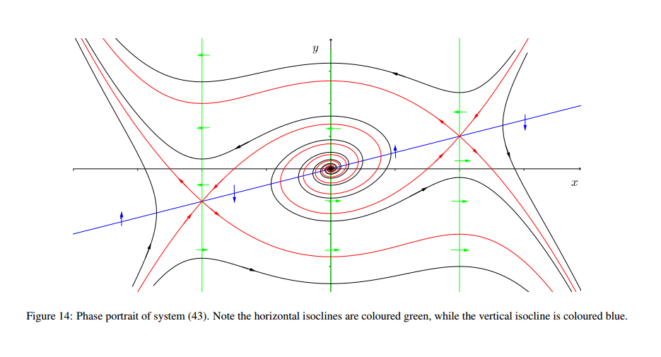
• A nullcline is a curve in the phase plane where one of the derivatives $\frac{dx}{dt}$ or $\frac{dy}{dt}$ is zero
  • The $x$-nullcline is the set of points where $\frac{dx}{dt} = 0$, and the $y$-nullcline is the set of points where $\frac{dy}{dt} = 0$
  • Nullclines divide the phase plane into regions where the signs of $\frac{dx}{dt}$ and $\frac{dy}{dt}$ remain constant
  • The intersection points of the $x$-nullcline and $y$-nullcline are equilibrium points of the system

Equilibrium Points and Stability

Classification of Equilibrium Points

• An equilibrium point $(x^*, y^*)$ is a point in the phase plane where the system remains stationary, i.e., $\frac{dx}{dt} = 0$ and $\frac{dy}{dt} = 0$
  • At an equilibrium point, the vector field vanishes, and trajectories do not move away from or towards the point
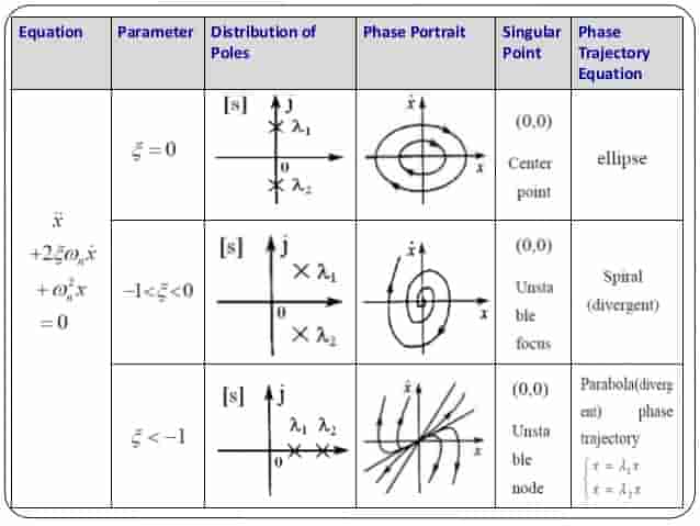
• Equilibrium points can be classified based on the behavior of nearby trajectories:
  • A stable equilibrium point attracts nearby trajectories, causing them to approach the point as $t \to \infty$
  • An unstable equilibrium point repels nearby trajectories, causing them to move away from the point as $t \to \infty$
  • A saddle point attracts trajectories along one direction and repels them along another direction

Determining Stability

• The stability of an equilibrium point can be determined by linearizing the system around the point and analyzing the eigenvalues of the Jacobian matrix
  • The Jacobian matrix $J(x^*, y^*)$ is the matrix of partial derivatives evaluated at the equilibrium point: $J = \begin{pmatrix} \frac{\partial f}{\partial x} & \frac{\partial f}{\partial y} \\ \frac{\partial g}{\partial x} & \frac{\partial g}{\partial y} \end{pmatrix}$
  • If both eigenvalues of $J(x^*, y^*)$ have negative real parts, the equilibrium point is stable (sink)
  • If both eigenvalues have positive real parts, the equilibrium point is unstable (source)
  • If one eigenvalue has a negative real part and the other has a positive real part, the equilibrium point is a saddle point