2.2 Wavefunctions and their physical interpretation

Wavefunction Properties

Fundamentals of Wavefunctions

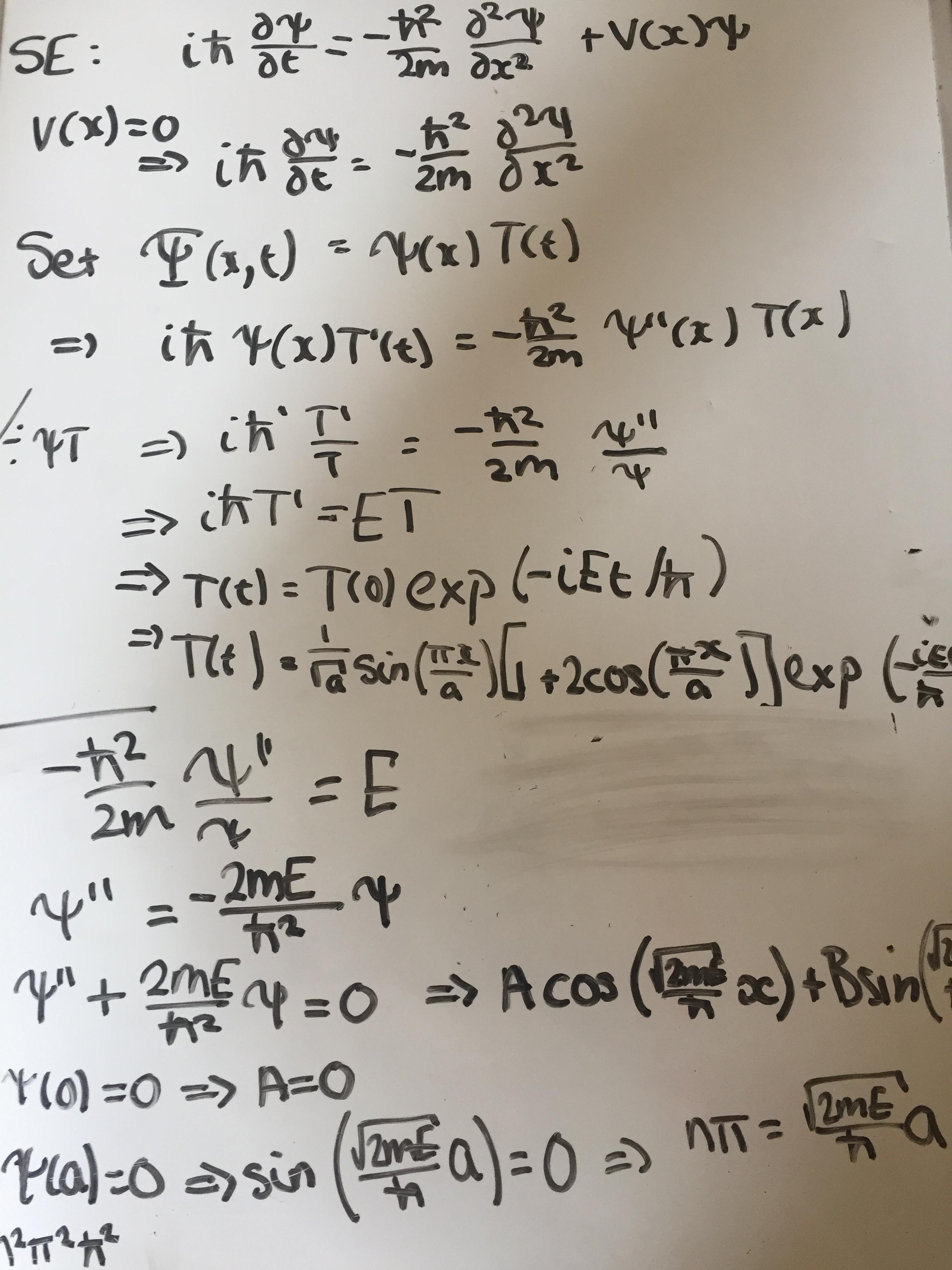
A wavefunction, denoted $\Psi(x, t)$, is a complex-valued function that completely describes the quantum state of a particle or system. It's the central object in quantum mechanics: once you know $\Psi$, you can extract every measurable property of the system.

Wavefunctions are solutions to the Schrödinger equation, which governs how quantum states evolve in time. Their physical meaning comes from the Born rule: the probability of finding a particle at a given location is proportional to $|\Psi(x, t)|^2$, the squared modulus of the wavefunction at that point. This is what connects the abstract math to actual lab measurements.

Because $\Psi$ is complex-valued, it has both an amplitude and a phase. The amplitude relates to probability, while the phase encodes information about how the wave oscillates across space and time. Phase differences between wavefunctions become physically important in interference and superposition.

Essential Properties of Wavefunctions

For a wavefunction to be physically meaningful, it must satisfy three conditions:

• Normalization: The total probability of finding the particle somewhere in all of space must equal 1. Mathematically:

$\int_{-\infty}^{\infty} |\Psi(x, t)|^2 \, dx = 1$

If this integral diverges or equals zero, the wavefunction doesn't represent a physical state. You often need to find a normalization constant to enforce this condition.

• Continuity: Both $\Psi$ and its first spatial derivative $\partial \Psi / \partial x$ must be continuous everywhere, except at points where the potential energy is infinite. This requirement comes from the Schrödinger equation itself: a discontinuous $\Psi$ or $\partial \Psi / \partial x$ would make the kinetic energy term blow up. The one exception is an infinite potential wall (like the boundaries of an infinite square well), where the derivative can be discontinuous.
• Single-valuedness: At every point in space, $\Psi$ must have exactly one value. If the wavefunction were multi-valued, the probability density would be ambiguous, and you couldn't make consistent predictions.

Probability from Wavefunctions

Probability Density and Its Calculation

The probability density is defined as:

$\rho(x, t) = |\Psi(x, t)|^2 = \Psi^*(x, t)\,\Psi(x, t)$

This quantity is always real and non-negative, which makes sense since it represents a probability per unit length (in 1D). It tells you how likely you are to find the particle near position $x$ at time $t$.

To find the probability of the particle being in a specific region between $x = a$ and $x = b$, integrate the probability density over that interval:

$P(a \leq x \leq b) = \int_a^b |\Psi(x, t)|^2 \, dx$

The limits depend on what you're asked. If you want the probability over all space, integrate from $-\infty$ to $+\infty$ (which gives 1 for a normalized wavefunction).

Probability Current and the Continuity Equation

Probability doesn't just sit still; it can flow through space. The probability current $J(x, t)$ quantifies this flow:

$J(x, t) = \frac{\hbar}{2mi}\left[\Psi^* \frac{\partial \Psi}{\partial x} - \Psi \frac{\partial \Psi^*}{\partial x}\right]$

Here $\hbar$ is the reduced Planck constant, $m$ is the particle mass, and $i$ is the imaginary unit. Despite the complex quantities involved, $J$ itself is real-valued. It tells you the rate at which probability is being transported past a point, and its sign indicates the direction of flow.

The probability current and density are linked by the continuity equation:

$\frac{\partial \rho(x, t)}{\partial t} + \frac{\partial J(x, t)}{\partial x} = 0$

This is a statement of conservation of probability: probability can't appear or disappear, it can only flow from one region to another. This is the quantum analogue of charge conservation in electromagnetism.

Wavefunctions and Measurables

Observables and Operators

Every measurable quantity (observable) in quantum mechanics corresponds to a Hermitian operator that acts on the wavefunction. Hermitian operators are guaranteed to have real eigenvalues, which is necessary since measurement outcomes are real numbers. Key examples:

• Position: $\hat{x}$ (multiply by $x$)
• Momentum: $\hat{p} = -i\hbar \frac{\partial}{\partial x}$
• Energy (Hamiltonian): $\hat{H} = -\frac{\hbar^2}{2m}\frac{\partial^2}{\partial x^2} + V(x)$

The expectation value of an observable $A$ gives the average result you'd obtain over many identical measurements on identically prepared systems:

$\langle A \rangle = \int_{-\infty}^{\infty} \Psi^*(x, t)\, \hat{A}\, \Psi(x, t) \, dx$

This is the bridge between the wavefunction formalism and experimental results.

Uncertainty Principle and Wavefunction Collapse

The Heisenberg uncertainty principle places a fundamental limit on how precisely you can simultaneously know two complementary observables. For position and momentum:

$\sigma_x \, \sigma_p \geq \frac{\hbar}{2}$

where $\sigma_x$ and $\sigma_p$ are the standard deviations of position and momentum. This isn't about measurement imperfections; it's built into the structure of wavefunctions. A wavefunction that's sharply localized in position (small $\sigma_x$) necessarily has a broad spread in momentum (large $\sigma_p$), and vice versa.

Wavefunction collapse describes what happens upon measurement. Before you measure, the system can exist in a superposition of eigenstates of the observable. When you perform the measurement, the wavefunction instantaneously reduces to the eigenstate corresponding to the result you obtained. After collapse, the system is in a definite state for that observable, and repeating the same measurement immediately will give the same result.

Wavefunction Behavior in Systems

Infinite Square Well

In the infinite square well (a particle confined between rigid walls at $x = 0$ and $x = L$), the wavefunctions are standing waves that vanish at both boundaries:

$\Psi_n(x) = \sqrt{\frac{2}{L}} \sin\left(\frac{n\pi x}{L}\right), \quad n = 1, 2, 3, \ldots$

The corresponding energy levels are quantized:

$E_n = \frac{n^2 \pi^2 \hbar^2}{2mL^2}$

Note that the ground state ($n = 1$) has nonzero energy, a direct consequence of the uncertainty principle. Each successive state has one additional node (zero crossing) inside the well.

Quantum Harmonic Oscillator

For the harmonic oscillator potential $V(x) = \frac{1}{2}m\omega^2 x^2$, the wavefunctions involve Hermite polynomials multiplied by a Gaussian envelope:

$\Psi_n(x) \propto H_n\left(\sqrt{\frac{m\omega}{\hbar}}\, x\right) \exp\left(-\frac{m\omega x^2}{2\hbar}\right)$

The energy levels are evenly spaced:

$E_n = \left(n + \frac{1}{2}\right)\hbar\omega, \quad n = 0, 1, 2, \ldots$

The ground state ($n = 0$) is a pure Gaussian, the most localized state possible. Excited states spread out further and develop additional nodes. The equal spacing $\hbar\omega$ between levels is a distinctive feature of this system.

Hydrogen Atom

The hydrogen atom wavefunctions separate into radial and angular parts, labeled by three quantum numbers:

• Principal quantum number $n$ ($n = 1, 2, 3, \ldots$): determines the energy and overall size of the orbital
• Angular momentum quantum number $l$ ($l = 0, 1, \ldots, n-1$): determines the shape (s, p, d, f for $l = 0, 1, 2, 3$)
• Magnetic quantum number $m_l$ ($m_l = -l, \ldots, +l$): determines the orientation in space

The angular parts are spherical harmonics $Y_l^{m_l}(\theta, \phi)$, and the radial parts involve associated Laguerre polynomials. The shell structure of atoms (and the periodic table) follows directly from these quantum numbers.

Quantum Tunneling

Tunneling occurs when a particle passes through a potential barrier that it classically wouldn't have enough energy to overcome. Inside the barrier, the wavefunction doesn't oscillate but instead decays exponentially:

$\Psi(x) \propto e^{-\kappa x}, \quad \text{where } \kappa = \frac{\sqrt{2m(V_0 - E)}}{\hbar}$

If the barrier is thin enough, the wavefunction hasn't fully decayed by the time it reaches the other side, giving a nonzero transmission probability. The tunneling probability decreases exponentially with both the barrier width and $\sqrt{V_0 - E}$, where $V_0$ is the barrier height and $E$ is the particle's energy.

Visualization Techniques

Plotting wavefunctions in different ways reveals different physical content:

• Real and imaginary parts of $\Psi(x, t)$ separately show the oscillatory character and phase relationships
• Probability density $|\Psi(x, t)|^2$ shows where the particle is most likely to be found, which is usually the most physically intuitive plot
• Probability current $J(x, t)$ reveals the direction and rate of probability flow, which is especially useful for scattering problems and tunneling

For bound states (like the square well or harmonic oscillator), the probability density is stationary in time for energy eigenstates. For superpositions of energy eigenstates, the probability density oscillates, and these time-dependent plots can build intuition about quantum dynamics.