5.3 Well hydraulics and pumping tests

Well Hydraulics

Principles of well hydraulics

Well hydraulics describes how groundwater flows toward a well during pumping. When you pump water out of a well, you lower the water level in and around it, creating a pressure gradient that drives flow inward from the surrounding aquifer.

Drawdown is the drop in water level caused by pumping. You measure it as the difference between the static water level (before pumping) and the current pumping water level. Drawdown increases with higher pumping rates and longer pumping durations, and it decreases with distance from the well.

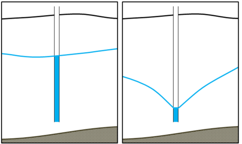
The cone of depression is the three-dimensional zone of lowered water levels that forms around a pumping well. Picture an inverted cone shape in the water table (or potentiometric surface), steepest near the well and flattening out with distance. Its shape and extent depend on aquifer permeability, porosity, pumping rate, and how long pumping continues.

Two aquifer properties control how drawdown develops:

• Transmissivity ($T$): the rate at which water is transmitted through a full aquifer thickness per unit width under a unit hydraulic gradient. Units are $m^2/day$ or $ft^2/day$. Higher transmissivity means the aquifer moves water more easily, so drawdown spreads out faster but stays shallower.
• Storativity ($S$): the volume of water released from storage per unit surface area per unit decline in hydraulic head (dimensionless). In confined aquifers, storativity is very small ($10^{-5}$ to $10^{-3}$), while in unconfined aquifers the equivalent value (specific yield) is much larger ($0.01$ to $0.30$).

Purpose of aquifer pumping tests

Pumping tests are the primary field method for determining aquifer properties ($T$, $S$, hydraulic conductivity) and well performance parameters (efficiency, specific capacity, radius of influence). The basic procedure is:

1. Install observation wells at known distances from the pumping well to monitor drawdown at multiple locations.
2. Measure pre-pumping static water levels in both the pumping well and all observation wells.
3. Pump the well at a constant rate for a sufficient duration, often 24 to 72 hours, to develop a clear drawdown response.
4. Record water levels in the pumping well and observation wells at increasing time intervals throughout pumping (e.g., every minute early on, then every 10 minutes, then hourly).
5. After pumping stops, continue measuring water levels during the recovery period as levels rise back toward static conditions.

The resulting time-drawdown data are then analyzed using curve-matching or graphical methods to estimate aquifer properties.

Pumping Test Analysis

Interpretation of pumping test data

Two classic methods are used to analyze pumping test data from confined aquifers under ideal (homogeneous, isotropic, infinite extent) conditions.

Theis Method

The Theis equation relates drawdown to pumping rate and aquifer properties:

$s = \frac{Q}{4\pi T} W(u)$

where $s$ is drawdown, $Q$ is the constant pumping rate, $T$ is transmissivity, and $W(u)$ is the Theis well function. The parameter $u$ is defined as:

$u = \frac{r^2 S}{4Tt}$

where $r$ is the distance from the pumping well, $S$ is storativity, and $t$ is time since pumping started.

Steps for the Theis curve-matching method:

1. Plot the type curve of $W(u)$ vs. $1/u$ on log-log paper.
2. Plot your observed data ($s$ vs. $t/r^2$, or $s$ vs. $t$) on a separate log-log sheet at the same scale.
3. Overlay the data plot on the type curve and shift it (keeping axes parallel) until the data points align with the curve.
4. Pick a match point and read off the corresponding values of $W(u)$, $1/u$, $s$, and $t$ (or $t/r^2$).
5. Solve for $T$ and $S$ using the Theis equation and the definition of $u$.

Cooper-Jacob Method

This is a simplification of the Theis solution that's valid when $u < 0.01$ (i.e., at sufficiently large times or small distances from the well). Under this condition, the well function can be approximated by a logarithmic expression, and the drawdown equation becomes:

$s = \frac{2.3Q}{4\pi T} \log_{10}\frac{2.25Tt}{r^2 S}$

Steps for the Cooper-Jacob method:

1. Plot drawdown ($s$) on a linear axis against time ($t$) on a logarithmic axis (semi-log plot).
2. Fit a straight line through the data points that fall in the valid range (where $u < 0.01$). Early-time data may deviate from the line.
3. Determine the slope of the line: the drawdown per log cycle ($\Delta s$). Calculate transmissivity as $T = \frac{2.3Q}{4\pi \Delta s}$.
4. Extend the straight line to where $s = 0$ and read off the corresponding time ($t_0$). Calculate storativity as $S = \frac{2.25Tt_0}{r^2}$.

The Cooper-Jacob method is often preferred in practice because it's simpler and avoids the subjectivity of type-curve matching.

Concepts in well performance

Well Efficiency measures how effectively a well converts the available drawdown into discharge. In a real well, the total drawdown has two components: aquifer loss (the theoretical drawdown from flow through the aquifer) and well loss (additional drawdown from friction and turbulent flow through the screen, gravel pack, and casing).

• Well efficiency = (theoretical aquifer drawdown / actual total drawdown) × 100%
• A well at 100% efficiency would have zero well losses, which never happens in practice. Efficiencies above 70-80% are generally considered good.
• Efficiency decreases over time as wells age due to screen clogging, encrustation, or biofouling.

Specific Capacity is the pumping rate divided by the drawdown in the well at a given time (typically after 24 hours of pumping). It's expressed in units like $gpm/ft$ or $m^3/day/m$.

• Specific capacity provides a quick, practical indicator of well productivity.
• It tends to decrease with increasing pumping rate (because well losses increase nonlinearly with discharge) and with longer pumping duration.
• It can be used to roughly estimate transmissivity, though the relationship depends on well efficiency and aquifer type.

Radius of Influence is the distance from the pumping well to the point where drawdown becomes negligible. It defines the outer boundary of the cone of depression.

• The radius of influence grows with pumping duration and pumping rate, and it's larger in high-transmissivity aquifers.
• It can be estimated from pumping test data or, for approximate calculations, using empirical formulas. For example, the Sichardt formula for unconfined aquifers: $R = 3000 \cdot s_w \cdot \sqrt{K}$, where $s_w$ is drawdown at the well and $K$ is hydraulic conductivity.
• Knowing the radius of influence is important for assessing potential interference between neighboring wells and impacts on nearby surface water bodies.