Spectral methods solve partial differential equations (PDEs) by representing solutions as combinations of global basis functions, typically trigonometric functions or orthogonal polynomials. Unlike finite difference or finite element approaches that use local approximations, spectral methods leverage the global structure of these basis functions to achieve exponential convergence for smooth problems. This makes them a go-to choice in CFD when high spatial accuracy matters, particularly in turbulence simulations and flows with periodic geometries.
Spectral methods overview
The core idea behind spectral methods is to express an unknown solution as a truncated series of known basis functions:
where are the expansion coefficients and are the basis functions (sines, cosines, Chebyshev polynomials, etc.). The PDE is then recast as a problem for the coefficients rather than for directly.
What makes spectral methods special is their convergence behavior. For smooth solutions, the approximation error decreases exponentially as you add more basis functions. Compare this to finite differences, where doubling the grid points only reduces error by a fixed algebraic factor. The tradeoff is that spectral methods work best on simple geometries and smooth problems. Discontinuities or sharp gradients can cause trouble (the Gibbs phenomenon), which is why these methods are often paired with other techniques for more complex scenarios.
Fourier series representations
Fourier series decompose periodic functions into sums of sines and cosines. In CFD, they're the natural choice whenever the flow repeats in one or more spatial directions.
Periodic functions
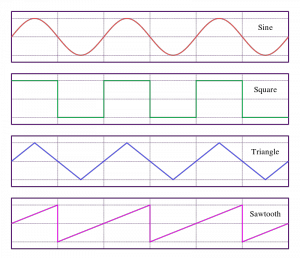
A function is periodic with period if for all . Classic examples include sine waves, square waves, and sawtooth waves. Many fluid dynamics problems have inherent periodicity: turbulent channel flow is often treated as periodic in the streamwise and spanwise directions, and flow around a cylinder can exploit azimuthal periodicity.
Trigonometric polynomials
A trigonometric polynomial approximates a periodic function using a finite number of sine and cosine terms:
Adding more terms improves the approximation. For smooth periodic functions, the improvement is dramatic: each additional term can reduce the error by a roughly constant factor, giving exponential convergence.
Fourier coefficients
The coefficients determine how much each frequency contributes to the overall signal. You compute them by projecting the function onto each basis function using an inner product, or more practically, by applying a fast Fourier transform (FFT).
The rate at which Fourier coefficients decay tells you about the smoothness of the function. Smooth functions have coefficients that drop off rapidly, which is exactly why spectral methods converge so fast for smooth problems. If the coefficients decay slowly, the function has sharp features that are harder to resolve.
Chebyshev polynomials
When the problem isn't periodic, Chebyshev polynomials are the most common spectral basis. They're defined on the interval and have approximation properties that are nearly optimal among all polynomial bases.
Orthogonal polynomials
Chebyshev polynomials belong to a broader family of orthogonal polynomials, which satisfy:
where is the Chebyshev weight function. Other families include Legendre polynomials (uniform weight) and Hermite polynomials (Gaussian weight on the real line). Orthogonality is what makes computing expansion coefficients straightforward and numerically stable.
Chebyshev nodes
Chebyshev nodes are the points where you sample the function for a Chebyshev expansion. They're defined as:
These points cluster near the endpoints of the interval . That clustering isn't a bug; it's a feature. It suppresses the Runge phenomenon (wild oscillations near boundaries that plague equally-spaced polynomial interpolation) and provides extra resolution near walls, which is exactly where boundary layers live in fluid flows.
Chebyshev differentiation matrices
To compute derivatives spectrally, you build a differentiation matrix such that if is the vector of function values at the Chebyshev nodes, then gives the derivative values at those same nodes.
These matrices are constructed from the analytic properties of Chebyshev polynomials and their derivatives. They're dense (every node influences every derivative value), which reflects the global nature of spectral approximations. Higher derivatives are obtained by applying repeatedly: gives the second derivative, and so on.
Spectral differentiation
Computing spatial derivatives accurately is central to solving PDEs. Spectral differentiation does this by operating on the expansion coefficients or by applying differentiation matrices to nodal values.
Differentiation matrices
For any spectral basis, you can construct a matrix that maps function values to derivative values at the collocation points. For Fourier methods, differentiation in coefficient space is especially clean: taking a derivative just multiplies the -th Fourier coefficient by , where is the wavenumber.
For Chebyshev methods, the differentiation matrix is dense, with entries determined by the Chebyshev nodes and the Lagrange interpolation formula. This density contrasts with finite difference stencils, which produce sparse, banded matrices.
Accuracy vs finite differences
The accuracy gap between spectral and finite difference methods is significant for smooth problems:
- Finite differences converge algebraically: the error scales as , where depends on the stencil order ( for second-order central differences, for fourth-order, etc.)
- Spectral methods converge exponentially: for some
In practice, this means a spectral method with 32 grid points can outperform a second-order finite difference method with thousands of points, provided the solution is smooth. This efficiency is why spectral methods dominate in direct numerical simulation (DNS) of turbulence, where resolving all scales accurately is critical.

Spectral integration
Computing integrals of spectrally represented functions follows a similar philosophy to differentiation: operate on the coefficients or use specialized quadrature rules.
Integration matrices
Just as differentiation matrices map function values to derivative values, integration matrices map function values to integral values. For Chebyshev expansions, the integration matrix relates the coefficients of a function to the coefficients of its antiderivative through a recurrence relation. These matrices tend to be simpler in structure than differentiation matrices.
Gaussian quadrature
Gaussian quadrature rules approximate integrals as weighted sums of function values at carefully chosen points:
The two most common variants in spectral methods are:
- Gauss-Chebyshev quadrature: uses Chebyshev nodes and the weight function
- Gauss-Legendre quadrature: uses Legendre nodes with uniform weight
A key property is that Gaussian quadrature with points integrates polynomials of degree up to exactly. This exactness is what underpins the accuracy of spectral methods when computing inner products and projection integrals.
Solving PDEs with spectral methods
The general workflow for solving a PDE with spectral methods involves these steps:
- Choose a basis appropriate to the boundary conditions (Fourier for periodic, Chebyshev for non-periodic)
- Expand the unknown in that basis with undetermined coefficients
- Substitute into the PDE and apply a projection method (Galerkin or collocation) to obtain equations for the coefficients
- Solve the resulting algebraic or ODE system for the coefficients
- Reconstruct the solution in physical space if needed
Poisson equation
The Poisson equation relates a scalar field to its source term through the Laplacian. It appears constantly in CFD: the pressure Poisson equation in incompressible flow, gravitational potential problems, and electrostatics.
In a Fourier basis, the Poisson equation becomes algebraic. Each Fourier mode decouples, and you simply divide each coefficient of by to get the corresponding coefficient of . This makes Fourier-based Poisson solvers extremely fast, especially when combined with FFTs.
Helmholtz equation
The Helmholtz equation generalizes the Poisson equation by adding a term proportional to itself. It arises in time-harmonic wave problems (acoustics, electromagnetics) and also appears when implicit time-stepping is applied to diffusion terms in the Navier-Stokes equations.
Spectral methods handle the Helmholtz equation efficiently because, like the Poisson equation, it decouples in Fourier space. Each mode satisfies , which is a simple algebraic equation.
Navier-Stokes equations
The incompressible Navier-Stokes equations consist of the momentum equation and the continuity (divergence-free) constraint:
Spectral methods have been the backbone of DNS since the 1970s. A typical approach treats the linear terms (viscous diffusion, pressure) implicitly in Fourier/Chebyshev space, while the nonlinear convective term is computed in physical space (a "pseudospectral" approach) and then transformed back. This avoids the expensive convolution sums that would arise from computing the nonlinear term directly in coefficient space.
Spectral element methods
Pure spectral methods struggle with complex geometries because global basis functions don't adapt well to irregular domains. Spectral element methods solve this by combining spectral accuracy with the geometric flexibility of finite elements.
Domain decomposition
The computational domain is divided into non-overlapping elements (quadrilaterals in 2D, hexahedra in 3D). Within each element, the solution is represented by a high-order polynomial expansion, typically using Legendre or Chebyshev polynomials on a reference element mapped to the physical element.
This decomposition allows you to handle complex geometries, refine the mesh locally where the flow has fine-scale features, and distribute work across processors for parallel computation.
Elemental operations
Within each element, you compute local mass matrices, stiffness matrices, and force vectors. These are the same types of matrices that appear in standard finite element methods, but the high-order polynomial basis gives spectral-level accuracy within each element.
Because elements are independent at this stage, elemental operations parallelize naturally. Each processor can handle its own set of elements without communicating with others.
Assembly of global system
After computing elemental contributions, you assemble them into a global system by enforcing continuity of the solution (and sometimes its derivatives) across element boundaries. The resulting global matrix is sparse because each element only connects to its immediate neighbors, unlike the dense matrices of pure spectral methods.
Standard sparse linear algebra solvers and preconditioners can then be applied to the global system. This combination of spectral accuracy within elements and sparse global structure is what makes spectral element methods practical for large-scale, geometrically complex CFD problems. Codes like Nek5000 and Nektar++ are built on this approach.
Fourier spectral methods
Fourier spectral methods are the simplest and most efficient spectral approach, but they require periodicity in at least one spatial direction.
Periodic boundary conditions
Periodicity means the solution satisfies in one or more directions. Fourier basis functions are inherently periodic, so periodic boundary conditions are enforced automatically without any special treatment. This is a significant advantage over methods that require explicit boundary condition implementation.
Common CFD applications with periodic boundaries include homogeneous turbulence (periodic in all three directions), channel flow (periodic in streamwise and spanwise directions), and mixing layers.
Fast Fourier transform (FFT)
The FFT is the algorithm that makes Fourier spectral methods practical. It computes the discrete Fourier transform of data points in operations instead of the required by direct summation.
For a 3D simulation on a grid, that's the difference between roughly and operations per transform. Since a typical time step requires multiple forward and inverse transforms, the FFT's efficiency is not just convenient but essential.
Dealiasing techniques
When you compute nonlinear terms (like ) in physical space and transform back to coefficient space, high-frequency products can "fold" back into the resolved frequency range. This is aliasing, and it introduces errors that can destabilize a simulation.
The most common fix is the 3/2 rule (also called zero-padding): before computing the nonlinear product, you pad the coefficient array with zeros to extend it to points, compute the product on this finer grid, then truncate back to modes. The equivalent approach from the other direction is the 2/3 rule, where you truncate the highest 1/3 of modes after the transform. Both achieve the same result. An alternative is spectral vanishing viscosity (SVV), which adds a small, spectrally-targeted dissipation to damp the high-frequency modes that would otherwise alias.
Spectral accuracy
Spectral accuracy refers to the exponential convergence that spectral methods achieve for smooth solutions. This is their defining advantage over lower-order methods.
Exponential convergence
For a smooth (infinitely differentiable) function, the error in a spectral approximation with modes decays as:
where depends on the analyticity properties of the solution. This means each additional mode reduces the error by a roughly constant factor, not a constant amount. For analytic functions (those that can be extended to the complex plane), convergence is even faster: the coefficients decay geometrically.
This exponential convergence breaks down when the solution has discontinuities or insufficient smoothness. In those cases, spectral methods revert to algebraic convergence and may exhibit Gibbs oscillations near the discontinuity.
Comparison to finite differences
| Property | Spectral Methods | Finite Differences |
|---|---|---|
| Convergence rate | Exponential () | Algebraic () |
| Basis functions | Global | Local |
| Matrix structure | Dense | Sparse/banded |
| Best suited for | Smooth solutions, simple geometries | General problems, complex geometries |
| Grid points needed for high accuracy | Few | Many |
For long-time integrations (e.g., climate modeling or turbulence statistics), the accuracy advantage of spectral methods compounds over thousands of time steps, making them strongly preferred when the geometry permits their use.
Implementation considerations
Getting spectral methods to perform well in practice requires attention to algorithmic efficiency, parallelization, and memory management.
Efficient algorithms
The most important algorithmic choice is using FFTs for Fourier-based methods. Beyond that, matrix-free operators avoid storing dense differentiation matrices explicitly by applying them through fast transforms. Iterative solvers (conjugate gradient, GMRES) with appropriate preconditioners are preferred over direct solvers for large systems, especially in 3D.
For Chebyshev methods, the fast cosine transform (a variant of the FFT) enables transformations between physical and coefficient space, avoiding the cost of direct matrix-vector multiplication.
Parallel computing
Spectral methods parallelize differently depending on the variant:
- Fourier methods: The FFT can be parallelized using slab or pencil decompositions, where the 3D grid is divided along one or two directions. Pencil decompositions scale better to large processor counts but require more communication.
- Spectral element methods: Parallelization is more natural because elements can be distributed across processors with communication only at shared boundaries.
Efficient parallel FFT libraries (FFTW, P3DFFT, 2DECOMP&FFT) are critical for scaling Fourier spectral methods to thousands of processors.
Memory requirements
Spectral methods tend to be more memory-intensive than low-order methods because:
- Dense differentiation and transformation matrices scale as per dimension
- Global basis functions mean every degree of freedom can couple to every other
Strategies to manage memory include matrix-free implementations (store only the data, apply operators via transforms), domain decomposition (spectral element methods break the global problem into smaller local ones), and out-of-core algorithms for very large problems. Despite these challenges, the high accuracy per degree of freedom often means spectral methods need far fewer total unknowns than a finite difference method for the same accuracy target, partially offsetting the higher per-unknown memory cost.