Confidence intervals for proportions are a crucial tool in statistical analysis. They allow us to estimate population parameters based on sample data, providing a range of plausible values with a specified level of confidence.
This topic explores how to construct and interpret confidence intervals for proportions. We'll cover the necessary conditions, calculation methods, and factors affecting interval width. Understanding these concepts is essential for making informed inferences about population characteristics.
Confidence intervals overview
- Confidence intervals provide a range of plausible values for an unknown population parameter based on sample data
- Allows for estimation and quantification of uncertainty in the estimate
Definition of confidence intervals
- A confidence interval is a range of values that is likely to contain the true population parameter with a certain level of confidence
- Consists of a point estimate (sample statistic) and a margin of error
- Represented as (lower bound, upper bound) or point estimate ± margin of error
Interpreting confidence intervals
- The confidence level (e.g., 95%) indicates the proportion of intervals that would contain the true population parameter if the sampling process were repeated many times
- A 95% confidence interval does not mean there is a 95% probability that the true parameter lies within the interval
- Interpret as "We are 95% confident that the true population parameter falls within this interval"
Confidence intervals for proportions
- Confidence intervals can be constructed for population proportions based on sample proportions
- Useful when working with categorical data or binary outcomes
Population proportion
- The population proportion, denoted as , represents the true proportion of individuals in the population with a specific characteristic
- Often unknown and estimated using sample data
Sample proportion
- The sample proportion, denoted as , is the proportion of individuals in a sample with a specific characteristic
- Calculated as , where is the number of individuals with the characteristic and is the sample size
- Used as a point estimate for the population proportion
Conditions for inference
- To construct a valid confidence interval for a proportion, certain conditions must be met:
- Random sampling: The sample should be randomly selected from the population
- Independence: The sample size should be less than 10% of the population size to ensure individual observations are independent
- Large sample size: The sample size should be large enough to approximate a normal distribution (generally, and )
Constructing confidence intervals
- The process of constructing a confidence interval involves determining the margin of error and combining it with the point estimate
Margin of error
- The margin of error represents the maximum likely difference between the sample proportion and the population proportion
- Calculated as the product of the critical value and the standard error of the sample proportion
- Formula: , where is the critical value
Critical values
- Critical values, denoted as , are derived from the standard normal distribution based on the desired confidence level
- Common critical values:
- 90% confidence level:
- 95% confidence level:
- 99% confidence level:
Confidence level
- The confidence level is the probability that the confidence interval will contain the true population parameter
- Commonly used confidence levels are 90%, 95%, and 99%
- Higher confidence levels result in wider intervals, while lower confidence levels result in narrower intervals
One vs two-sided intervals
- Confidence intervals can be one-sided or two-sided
- One-sided intervals provide a bound in only one direction (upper or lower)
- Two-sided intervals provide both an upper and lower bound
- Two-sided intervals are more common and provide a range of plausible values for the parameter
Factors affecting interval width
- Several factors influence the width of a confidence interval
Sample size
- Larger sample sizes generally lead to narrower confidence intervals
- As the sample size increases, the standard error decreases, resulting in a smaller margin of error
Confidence level
- Higher confidence levels (e.g., 99%) result in wider intervals compared to lower confidence levels (e.g., 90%)
- Increasing the confidence level requires a larger critical value, which increases the margin of error
Population proportion
- The width of the interval is affected by the variability in the population
- Proportions closer to 0.5 result in wider intervals compared to proportions near 0 or 1
- Maximum variability occurs when
Calculating confidence intervals
- The process of calculating confidence intervals involves using the standard normal distribution and finding critical z-values
Using standard normal distribution
- The standard normal distribution, denoted as , is a continuous probability distribution with a mean of 0 and a standard deviation of 1
- Used to find critical z-values based on the desired confidence level
- The area under the standard normal curve corresponds to probabilities
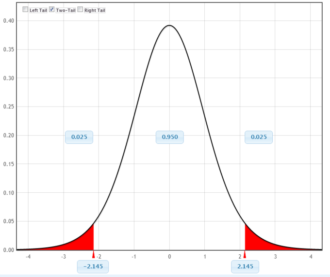
Finding critical z-values
- Critical z-values are the z-scores that correspond to the desired confidence level
- For a two-sided interval, the critical z-value is the z-score that separates the middle area (confidence level) from the tail areas
- Can be found using a standard normal table or statistical software
Confidence interval formula
- The confidence interval for a proportion is given by:
- is the sample proportion
- is the critical z-value based on the confidence level
- is the sample size
Interpreting results
- Interpreting confidence intervals involves considering both statistical and practical significance
Statistical vs practical significance
- Statistical significance refers to whether the results are unlikely to have occurred by chance alone
- Practical significance considers the magnitude and importance of the results in the real-world context
- A statistically significant result may not always be practically significant
Limitations of confidence intervals
- Confidence intervals have some limitations to consider:
- They do not provide information about the shape of the distribution
- They are sensitive to violations of assumptions (e.g., non-random sampling)
- They do not account for other sources of bias or error in the study design or data collection

Confidence intervals vs hypothesis tests
- Confidence intervals and hypothesis tests are related but distinct statistical methods
Similarities and differences
- Both methods use sample data to make inferences about population parameters
- Confidence intervals provide a range of plausible values for the parameter, while hypothesis tests assess the evidence against a specific null hypothesis
- Confidence intervals do not involve a formal decision rule, while hypothesis tests result in a decision to reject or fail to reject the null hypothesis
When to use each approach
- Confidence intervals are appropriate when the goal is to estimate the value of a population parameter
- Hypothesis tests are used when the goal is to assess the evidence against a specific claim or hypothesis
- Confidence intervals can be used to complement hypothesis tests by providing additional information about the magnitude and precision of the estimate
Common misinterpretations
- It is important to avoid common misinterpretations of confidence intervals
Misunderstanding confidence level
- The confidence level is often misinterpreted as the probability that the true parameter lies within the interval
- The correct interpretation is that if the sampling process were repeated many times, the proportion of intervals containing the true parameter would be equal to the confidence level
Misinterpreting interval width
- A narrow interval does not necessarily imply a precise estimate or a large sample size
- The width of the interval is influenced by multiple factors, including the variability in the population and the desired confidence level
- It is important to consider the context and practical significance of the interval width
Worked examples
- Worked examples help illustrate the process of calculating and interpreting confidence intervals
Calculating intervals step-by-step
- Example: A survey of 500 adults found that 60% support a new policy. Construct a 95% confidence interval for the proportion of adults in the population who support the policy.
- Identify the sample proportion:
- Determine the critical z-value for a 95% confidence level:
- Calculate the margin of error:
- Construct the confidence interval: or
- Interpret the results: We are 95% confident that the true proportion of adults who support the policy is between 0.5576 and 0.6424.
Real-world applications
- Confidence intervals are widely used in various fields, such as:
- Medical research: Estimating the effectiveness of a treatment or the prevalence of a disease
- Marketing: Estimating the proportion of customers who prefer a specific product
- Political polls: Estimating the proportion of voters who support a candidate or policy
Practice problems
- Practice problems help reinforce understanding and application of confidence intervals
Varied difficulty levels
- Include practice problems with different difficulty levels to cater to learners at various stages of understanding
- Start with basic problems that focus on calculating intervals and gradually progress to more complex problems involving interpretation and real-world scenarios
Detailed solutions
- Provide detailed, step-by-step solutions for each practice problem
- Explain the reasoning behind each step and highlight key concepts
- Include interpretations of the results and discuss any relevant assumptions or considerations