10.1 Advanced topics in differential equations

Nonlinear differential equations are tricky beasts. They can have multiple solutions, or none at all. This section dives into the nitty-gritty of when and why solutions exist, and how to find them.

We'll also look at systems of equations and stability. Understanding these concepts helps us predict how complex systems behave over time. It's like having a crystal ball for math!

Solutions of Nonlinear Differential Equations

Existence and Uniqueness of Solutions

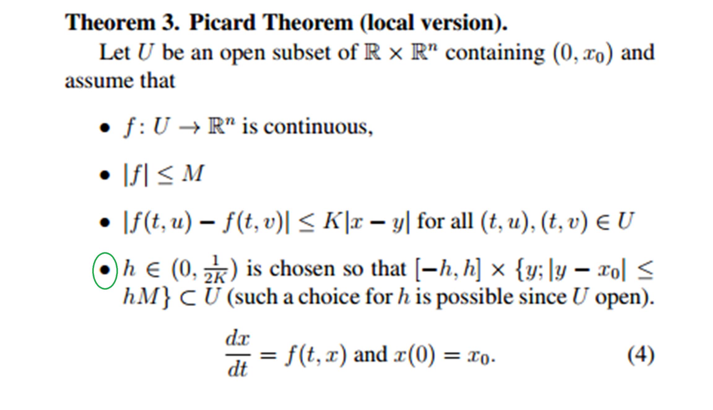
• The Picard-Lindelöf theorem, also known as the Cauchy-Lipschitz theorem, guarantees the existence and uniqueness of solutions to initial value problems for first-order nonlinear differential equations under certain conditions
• The conditions for the Picard-Lindelöf theorem include:
  • The continuity of the function $f(t, y)$ in the differential equation $\frac{dy}{dt} = f(t, y)$
  • The Lipschitz continuity of $f(t, y)$ with respect to $y$
• The Lipschitz condition ensures that the solutions of the differential equation do not diverge too quickly, which is essential for proving the uniqueness of solutions
• Example: The differential equation $\frac{dy}{dt} = y^2$ with the initial condition $y(0) = 1$ satisfies the conditions of the Picard-Lindelöf theorem and has a unique solution $y(t) = \frac{1}{1-t}$ for $t < 1$

Solution Methods for Nonlinear Differential Equations

• The contraction mapping principle is a key tool in proving the Picard-Lindelöf theorem and establishing the existence and uniqueness of solutions
• The Picard iteration method is a constructive approach to finding the solution of a nonlinear differential equation, which involves iteratively approximating the solution using a sequence of functions
  • The Picard iteration starts with an initial approximation $y_0(t)$ and generates a sequence of functions $y_n(t)$ that converge to the actual solution $y(t)$
  • Each iteration is defined by $y_{n+1}(t) = y_0 + \int_{t_0}^t f(s, y_n(s)) ds$, where $y_0$ is the initial condition and $t_0$ is the initial time
• Example: Applying the Picard iteration method to the differential equation $\frac{dy}{dt} = t + y$ with the initial condition $y(0) = 1$ yields the sequence of approximations $y_0(t) = 1$, $y_1(t) = 1 + t + \frac{t^2}{2}$, $y_2(t) = 1 + t + \frac{t^2}{2} + \frac{t^3}{6}$, and so on, which converge to the exact solution $y(t) = 2e^t - t - 1$

Systems of Linear Differential Equations

Matrix Representation and General Solution

• A system of linear differential equations can be represented in matrix form as $\mathbf{x}'(t) = A\mathbf{x}(t)$, where $\mathbf{x}(t)$ is a vector of functions and $A$ is a constant matrix
• The general solution of a system of linear differential equations can be expressed as a linear combination of exponential functions, where the exponents are the eigenvalues of the matrix $A$
• The general solution of the system can be written as $\mathbf{x}(t) = c_1\mathbf{v}_1e^{\lambda_1t} + c_2\mathbf{v}_2e^{\lambda_2t} + \ldots + c_n\mathbf{v}_ne^{\lambda_nt}$, where:
  • $c_i$ are arbitrary constants
  • $\mathbf{v}_i$ are the eigenvectors corresponding to each eigenvalue
  • $\lambda_i$ are the corresponding eigenvalues
• Example: Consider the system of linear differential equations $\frac{dx}{dt} = 2x + y$, $\frac{dy}{dt} = x + 2y$. The matrix representation is $\mathbf{x}'(t) = \begin{pmatrix} 2 & 1 \\ 1 & 2 \end{pmatrix}\mathbf{x}(t)$. The eigenvalues are $\lambda_1 = 3$ and $\lambda_2 = 1$, and the corresponding eigenvectors are $\mathbf{v}_1 = \begin{pmatrix} 1 \\ 1 \end{pmatrix}$ and $\mathbf{v}_2 = \begin{pmatrix} -1 \\ 1 \end{pmatrix}$. The general solution is $\mathbf{x}(t) = c_1\begin{pmatrix} 1 \\ 1 \end{pmatrix}e^{3t} + c_2\begin{pmatrix} -1 \\ 1 \end{pmatrix}e^{t}$

Eigenvalues and Eigenvectors

• Eigenvalues and eigenvectors of the matrix $A$ play a crucial role in determining the behavior and stability of the solutions to the system of linear differential equations
• The eigenvalues of the matrix $A$ can be found by solving the characteristic equation $\det(A - \lambda I) = 0$, where $\lambda$ represents the eigenvalues and $I$ is the identity matrix
• The eigenvectors corresponding to each eigenvalue can be found by solving the equation $(A - \lambda I)\mathbf{v} = \mathbf{0}$, where $\mathbf{v}$ represents the eigenvectors
• The eigenvalues determine the growth or decay of the solutions, while the eigenvectors determine the direction of the solutions in the phase space
• Example: For the matrix $A = \begin{pmatrix} 1 & 2 \\ 3 & 4 \end{pmatrix}$, the characteristic equation is $\det\begin{pmatrix} 1-\lambda & 2 \\ 3 & 4-\lambda \end{pmatrix} = (1-\lambda)(4-\lambda) - 6 = \lambda^2 - 5\lambda - 2 = 0$. The eigenvalues are $\lambda_1 = -1$ and $\lambda_2 = 2$. The corresponding eigenvectors are $\mathbf{v}_1 = \begin{pmatrix} -2 \\ 1 \end{pmatrix}$ and $\mathbf{v}_2 = \begin{pmatrix} 1 \\ 1 \end{pmatrix}$

Laplace Transform for Initial Value Problems

Definition and Properties of the Laplace Transform

• The Laplace transform is an integral transform that converts a function of time, $f(t)$, into a function of a complex variable, $F(s)$, in the frequency domain
• The Laplace transform of a function $f(t)$ is defined as $\mathcal{L}\{f(t)\} = F(s) = \int_0^{\infty} f(t)e^{-st} dt$, where $s$ is a complex variable
• The Laplace transform has several important properties, such as linearity, scaling, shifting, differentiation, and integration, which facilitate the manipulation of transformed functions
• Example: The Laplace transform of the exponential function $f(t) = e^{at}$ is $\mathcal{L}\{e^{at}\} = \frac{1}{s-a}$ for $\text{Re}(s) > a$

Solving Initial Value Problems using the Laplace Transform

• The Laplace transform is particularly useful for solving initial value problems involving higher-order linear differential equations with constant coefficients
• The Laplace transform of the nth derivative of a function $f(t)$ is given by $\mathcal{L}\{f^{(n)}(t)\} = s^nF(s) - s^{n-1}f(0) - s^{n-2}f'(0) - \ldots - f^{(n-1)}(0)$, where $f(0)$, $f'(0)$, ..., $f^{(n-1)}(0)$ are the initial conditions
• By taking the Laplace transform of a linear differential equation, the equation is transformed into an algebraic equation in terms of $F(s)$, which can be solved for $F(s)$ using algebraic manipulation
• The solution in the time domain, $f(t)$, can be obtained by applying the inverse Laplace transform to $F(s)$ using techniques such as partial fraction decomposition, the convolution theorem, or tables of Laplace transforms
• Example: Consider the initial value problem $y'' + 4y' + 3y = 0$, $y(0) = 1$, $y'(0) = 0$. Taking the Laplace transform yields $(s^2 + 4s + 3)Y(s) - sy(0) - y'(0) = 0$, where $Y(s) = \mathcal{L}\{y(t)\}$. Substituting the initial conditions and solving for $Y(s)$ gives $Y(s) = \frac{s+4}{(s+1)(s+3)}$. Using partial fraction decomposition and the inverse Laplace transform, the solution in the time domain is $y(t) = \frac{3}{2}e^{-t} - \frac{1}{2}e^{-3t}$

Stability of Equilibrium Points

Concept of Stability

• Stability refers to the behavior of solutions to a nonlinear system near equilibrium points, which are the points where the rate of change of the system variables is zero
• An equilibrium point is stable if nearby solutions remain close to the equilibrium point as time progresses, while an unstable equilibrium point is one where nearby solutions diverge from the equilibrium point over time
• The stability of an equilibrium point can be classified as:
  • Asymptotically stable: Nearby solutions converge to the equilibrium point as time approaches infinity
  • Stable: Nearby solutions remain close to the equilibrium point but may not converge to it
  • Unstable: Nearby solutions diverge from the equilibrium point over time
• Example: Consider the nonlinear system $\frac{dx}{dt} = -x(1-x)$, $\frac{dy}{dt} = -y$. The equilibrium points are $(0, 0)$ and $(1, 0)$. The point $(0, 0)$ is unstable, while the point $(1, 0)$ is asymptotically stable

Methods for Analyzing Stability

• Lyapunov stability theory provides a framework for analyzing the stability of equilibrium points without explicitly solving the nonlinear system
  • Lyapunov functions are scalar-valued functions that can be used to determine the stability of an equilibrium point based on the sign of the function's time derivative along the system trajectories
  • If a Lyapunov function exists and its time derivative is negative definite (or negative semidefinite for stability), then the equilibrium point is stable (or asymptotically stable)
• The linearization method involves approximating the nonlinear system near an equilibrium point using a linear system and analyzing the stability of the linearized system using eigenvalues of the Jacobian matrix
  • The Jacobian matrix is the matrix of partial derivatives of the system functions evaluated at the equilibrium point
  • If the real parts of all eigenvalues of the Jacobian matrix are negative, the equilibrium point is asymptotically stable; if at least one eigenvalue has a positive real part, the equilibrium point is unstable
• Example: For the nonlinear system $\frac{dx}{dt} = -x + xy$, $\frac{dy}{dt} = -y + x^2$, the equilibrium points are $(0, 0)$ and $(1, 1)$. Using the linearization method, the Jacobian matrix at $(0, 0)$ is $\begin{pmatrix} -1 & 0 \\ 0 & -1 \end{pmatrix}$, which has negative eigenvalues, indicating that $(0, 0)$ is asymptotically stable. The Jacobian matrix at $(1, 1)$ is $\begin{pmatrix} 0 & 1 \\ 2 & -1 \end{pmatrix}$, which has one positive and one negative eigenvalue, indicating that $(1, 1)$ is unstable

Solutions Near Singular Points

Classification of Singular Points

• Singular points, also known as critical points or equilibrium points, are points in the phase space where the rate of change of the system variables is zero
• The behavior of solutions near singular points can be classified into different types based on the eigenvalues of the Jacobian matrix evaluated at the singular point:
  • Node: Both eigenvalues are real and have the same sign (stable node if negative, unstable node if positive)
  • Saddle: Both eigenvalues are real, but one is positive and the other is negative
  • Center: Both eigenvalues are purely imaginary (stable, but not asymptotically stable)
  • Spiral: Both eigenvalues are complex with nonzero real and imaginary parts (stable spiral if the real part is negative, unstable spiral if the real part is positive)
• Example: Consider the system $\frac{dx}{dt} = x - y$, $\frac{dy}{dt} = x + y$. The singular point is $(0, 0)$. The Jacobian matrix at $(0, 0)$ is $\begin{pmatrix} 1 & -1 \\ 1 & 1 \end{pmatrix}$, which has eigenvalues $\lambda_1 = 1 + i$ and $\lambda_2 = 1 - i$. Since the eigenvalues are complex with a positive real part, the singular point is an unstable spiral

Phase Portraits and Bifurcations

• The phase portrait is a graphical representation of the trajectories of a dynamical system in the phase space, which provides a qualitative understanding of the system's behavior
• Constructing a phase portrait involves:
  • Identifying the singular points
  • Determining their stability
  • Sketching the trajectories in the phase space based on the eigenvalues and eigenvectors of the Jacobian matrix
• Nullclines, which are curves in the phase space where one of the system variables has a zero rate of change, can be used to locate singular points and understand the flow of trajectories in the phase portrait
• Bifurcations, which are qualitative changes in the phase portrait as a parameter of the system varies, can be studied to understand how the behavior of the system changes with respect to the parameter
  • Examples of bifurcations include saddle-node bifurcation, pitchfork bifurcation, and Hopf bifurcation
• Example: The system $\frac{dx}{dt} = \mu x - x^3$, $\frac{dy}{dt} = -y$, where $\mu$ is a parameter, exhibits a pitchfork bifurcation at $\mu = 0$. For $\mu < 0$, there is one stable equilibrium point at $(0, 0)$. For $\mu > 0$, the point $(0, 0)$ becomes unstable, and two new stable equilibrium points appear at $(\pm\sqrt{\mu}, 0)$