3.2 Expected value and variance

Definition of expected value

Expected value gives you a single number that represents the "average" outcome of an uncertain event, weighted by how likely each outcome is. In finance, this is how you estimate potential returns on investments, price derivatives like options and futures, and compare different strategies on equal footing.

Probability-weighted average

For a discrete random variable, expected value is the sum of every possible outcome multiplied by its probability:

$E[X] = \sum_{i=1}^{n} x_i \cdot p(x_i)$

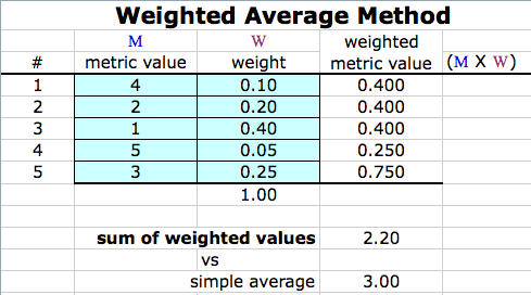
Think of it as a weighted average where the weights are probabilities. If a stock has a 60% chance of returning +10% and a 40% chance of returning -5%, the expected return is:

$E[X] = (0.60)(10\%) + (0.40)(-5\%) = 4\%$

The result is a single value representing the central tendency of the distribution. It doesn't tell you what will happen, but it tells you what to expect on average over many repetitions.

Applications in finance

• Derivative pricing: The fair price of options and futures is derived from the expected value of their payoffs (discounted to present value)
• Investment comparison: Expected value lets you rank opportunities by their average payoff, even when the underlying distributions look very different
• Trading strategies: Quantifying expected profit or loss per trade helps determine whether a strategy is worth pursuing
• Risk assessment: Combined with variance, expected value helps analysts gauge both the reward and the uncertainty of financial outcomes

Calculation of expected value

The calculation method depends on whether your random variable is discrete (countable outcomes) or continuous (outcomes across a range). You need both approaches for real-world financial modeling.

Discrete random variables

Use this when outcomes are countable, such as credit ratings, default/no-default scenarios, or a finite set of projected stock prices.

Formula: $E[X] = \sum_{i=1}^{n} x_i \cdot p(x_i)$

where $x_i$ is each possible outcome and $p(x_i)$ is its probability.

Steps:

1. List every possible outcome $x_i$
2. Assign each outcome its probability $p(x_i)$ (these must sum to 1)
3. Multiply each outcome by its probability
4. Sum all the products

For example, suppose a bond has three possible year-end scenarios: full repayment ($1,000) with probability 0.85, partial recovery ($400) with probability 0.10, and total default ($0) with probability 0.05.

$E[X] = (1000)(0.85) + (400)(0.10) + (0)(0.05) = 850 + 40 + 0 = 890$

The expected payoff is $890.

Continuous random variables

Use this when outcomes span a continuous range, such as asset returns, interest rates, or stock price movements.

Formula: $E[X] = \int_{-\infty}^{\infty} x \cdot f(x) \, dx$

where $f(x)$ is the probability density function (PDF).

Instead of summing over discrete outcomes, you integrate the product of each value and its density across the entire range. This is essential for modeling phenomena where outcomes aren't neatly countable, like the continuously distributed returns assumed in many asset pricing models.

Properties of expected value

These properties let you break complex problems into simpler pieces. They come up constantly in portfolio analysis and financial modeling.

Linearity of expectation

This is the most useful property. The expected value of a linear combination of random variables equals the linear combination of their expected values:

$E[aX + bY] = aE[X] + bE[Y]$

where $a$ and $b$ are constants.

This holds regardless of whether $X$ and $Y$ are independent. That's what makes it so powerful.

In portfolio terms: if you invest 60% in Asset A (expected return 8%) and 40% in Asset B (expected return 5%), the portfolio's expected return is:

$E[R_p] = (0.60)(8\%) + (0.40)(5\%) = 6.8\%$

You can decompose any portfolio's expected return into the weighted sum of individual asset expected returns.

Expected value of constants

The expected value of a constant is just the constant itself:

$E[c] = c$

This makes sense because there's no uncertainty in a fixed value. In practice, this simplifies calculations when your model includes fixed costs, guaranteed coupon payments, or other non-random components. You can separate the fixed and variable parts, calculate the expected value of the variable part, and add the constant back in.

Definition of variance

Variance measures how spread out a random variable's outcomes are around its expected value. In finance, variance is the standard way to quantify risk or volatility. A higher variance means outcomes are more dispersed, which translates to greater uncertainty about actual returns.

Measure of dispersion

Variance calculates the average squared deviation from the mean:

$Var(X) = E[(X - E[X])^2]$

Why squared? Squaring ensures that deviations above and below the mean don't cancel each other out. The tradeoff is that variance is expressed in squared units (e.g., "percent squared" for returns), which isn't very intuitive. That's why you'll often see standard deviation ($\sigma = \sqrt{Var(X)}$), which converts back to the original units.

A larger variance means the outcomes are more volatile. For two investments with the same expected return, a risk-averse investor would prefer the one with lower variance.

Relationship to expected value

There's a computational shortcut that's often easier to use than the definition:

$Var(X) = E[X^2] - (E[X])^2$

Steps to use this formula:

1. Calculate $E[X]$, the expected value
2. Calculate $E[X^2]$, the expected value of the squared outcomes
3. Subtract $(E[X])^2$ from $E[X^2]$

Using the bond example from earlier (outcomes: $1,000, $400, $0 with probabilities 0.85, 0.10, 0.05):

• $E[X] = 890$ (calculated above)
• $E[X^2] = (1000^2)(0.85) + (400^2)(0.10) + (0^2)(0.05) = 850{,}000 + 16{,}000 + 0 = 866{,}000$
• $Var(X) = 866{,}000 - (890)^2 = 866{,}000 - 792{,}100 = 73{,}900$

The variance is 73,900 (in dollars squared). The standard deviation would be $\sqrt{73{,}900} \approx \$271.85$, giving you a more interpretable measure of the payoff's uncertainty.