11.4 Data Analysis and Interpretation in Environmental Chemistry

Statistical Analysis of Environmental Data

Environmental chemistry generates messy, complex datasets. Statistical analysis gives you the tools to extract meaningful conclusions from that complexity, determine whether observed differences are real or just noise, and make defensible decisions about environmental quality.

Significance Testing and Reliability Assessment

The core question in most environmental studies is: Is this difference or trend real, or could it be due to chance? Statistical tests help you answer that.

Common hypothesis tests each serve a different purpose:

• T-tests compare means between two groups (e.g., upstream vs. downstream pollutant concentrations)
• ANOVA extends this comparison to three or more groups (e.g., contaminant levels across multiple sampling sites)
• Regression analysis quantifies relationships between variables and identifies trends over time

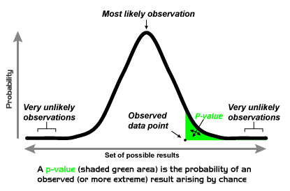
Confidence intervals give you a range of plausible values for a parameter, while p-values tell you the probability of observing your results if there were truly no effect. A p-value below your chosen threshold (typically 0.05) suggests the result is statistically significant, but always pair this with practical significance. A statistically significant difference of 0.001 ppb may not matter for environmental decision-making.

Sample size and power analysis should be planned before data collection. Power analysis helps you determine how many samples you need to reliably detect a meaningful difference. Too few samples and you risk missing real effects; too many wastes resources.

A few additional considerations for environmental datasets:

• Outliers are common and can dramatically skew results. Before removing them, investigate whether they represent real contamination events, instrument errors, or natural variability.
• Measurement uncertainty should be quantified using error propagation for simple calculations or Monte Carlo simulations for more complex models where analytical solutions aren't practical.
• Non-parametric tests (like the Mann-Whitney U or Kruskal-Wallis test) are often necessary because environmental data frequently violate normality assumptions due to skewed distributions or detection limits.
• Type I errors (false positives) mean declaring contamination when none exists, potentially wasting cleanup resources. Type II errors (false negatives) mean missing real contamination, potentially leaving communities exposed. Understanding this tradeoff is critical when setting significance thresholds for environmental decisions.

Advanced Statistical Techniques for Environmental Data

Environmental systems involve many interacting variables measured over space and time. Basic tests often aren't enough.

• Multivariate analysis (e.g., principal component analysis, factor analysis) reduces high-dimensional datasets to their most important underlying patterns. PCA, for instance, can help identify distinct pollution sources contributing to a mix of contaminants at a site.
• Time series analysis detects trends, seasonal cycles, and anomalies in long-term monitoring records. Techniques like the Mann-Kendall test are specifically designed for trend detection in environmental data that may not be normally distributed.
• Bayesian approaches let you formally incorporate prior knowledge (e.g., known background concentrations) and update your estimates as new monitoring data arrive. This is especially useful when sample sizes are small.
• Spatial statistics (e.g., kriging, variograms) account for the fact that nearby measurements tend to be more similar than distant ones. Ignoring spatial autocorrelation can lead to artificially inflated confidence in your results.
• Bootstrap and jackknife methods estimate uncertainty by resampling your existing data, which is valuable when you can't assume a particular distribution for your measurements.
• Meta-analysis combines results from multiple independent studies to draw stronger overall conclusions, such as synthesizing dozens of studies on mercury levels in freshwater fish across a region.
• Machine learning algorithms (random forests, neural networks, support vector machines) can identify complex nonlinear patterns in large datasets and make predictions, though interpretability can be a challenge compared to traditional statistical models.

Data Visualization for Environmental Communication

A well-chosen visualization can reveal patterns that tables of numbers never will. It can also mislead if done poorly. The goal is always clarity and honest representation of the data.

Effective Data Visualization Principles

Choosing the right chart type matters more than making it look fancy:

• Scatter plots show relationships between two continuous variables (e.g., dissolved oxygen vs. temperature)
• Line graphs display trends over time (e.g., monthly ozone concentrations over a decade)
• Bar charts compare discrete categories (e.g., average lead levels across different neighborhoods)
• Box plots and violin plots show the distribution and variability of data, not just the mean. Violin plots add density information that box plots miss.
• Error bars should always accompany point estimates to communicate uncertainty honestly

Geographic information systems (GIS) are essential for spatial environmental data. Mapping contaminant concentrations across a watershed, for example, can reveal spatial patterns and hotspots that summary statistics alone would obscure.

For time series data, pay attention to scale choices. A compressed y-axis can make a real trend look flat, while a stretched axis can make noise look like a crisis.

Best practices for all environmental visualizations:

• Use colorblind-friendly palettes (avoid red-green combinations)
• Label axes clearly with units
• Don't truncate axes in misleading ways
• Annotate key events (e.g., a policy change or spill event) directly on temporal plots

Advanced Visualization Techniques

When datasets become more complex, you need more sophisticated tools:

• Heatmaps and contour plots display spatial distributions of variables like soil contamination or temperature across a landscape. Color gradients represent concentration levels, making hotspots immediately visible.
• Network diagrams illustrate relationships between environmental components, such as how different pollutants co-occur or how species interact in a food web.
• Parallel coordinate plots let you visualize many variables simultaneously. Each vertical axis represents a different parameter, and each sample is a line connecting its values across all axes. This is useful for spotting clusters or outliers in high-dimensional data.
• Animated visualizations show how environmental conditions change over time, such as the seasonal expansion and contraction of a hypoxic zone.
• Dashboards combine multiple visualizations into a single interactive interface, allowing stakeholders to explore data at different scales and time periods.
• 3D visualizations can represent features like groundwater contaminant plumes or atmospheric dispersion patterns, though they should be used carefully since 3D perspectives can distort perception of values.
• Infographics distill complex findings into accessible summaries for policymakers and the public. These prioritize key takeaways over technical detail.

Environmental Data Interpretation for Risk Assessment

Collecting and analyzing data only matters if you can interpret it in a meaningful regulatory and health context. This section connects analytical results to real-world decisions.

Regulatory Standards and Compliance Assessment

Environmental regulations set legally enforceable limits for pollutant concentrations. Your job as an environmental chemist is to compare monitoring data against these benchmarks.

Key U.S. regulations and what they cover:

• The Clean Air Act sets National Ambient Air Quality Standards (NAAQS) for criteria pollutants like $\text{O}_3$, $\text{PM}_{2.5}$, $\text{SO}_2$, $\text{NO}_2$, CO, and lead
• The Clean Water Act establishes water quality criteria for surface waters, including limits on parameters like dissolved metals, nutrients, and pH
• The Safe Drinking Water Act sets Maximum Contaminant Levels (MCLs) for drinking water, such as 15 ppb for lead at the tap (action level) or 10 ppb for arsenic

Compliance assessment goes beyond simply checking whether a single measurement exceeds a standard. You need to consider:

• Exceedance frequency and duration: How often and for how long are standards exceeded? Many standards are based on averages (e.g., the annual $\text{PM}_{2.5}$ standard of 12 µg/m³) rather than single measurements.
• Background levels: Natural concentrations of some substances (e.g., arsenic in certain geologic formations) may approach or exceed regulatory limits, which affects how you interpret exceedances.
• Cumulative impacts: When multiple pollutants are present simultaneously, their combined effect may be greater than any single pollutant alone, even if each individual concentration is below its respective standard.
• Long-term trend analysis: Comparing monitoring data across years helps evaluate whether environmental policies are actually working. A declining trend in sulfate deposition after acid rain regulations, for example, demonstrates policy effectiveness.

Risk Assessment and Decision-Making

Environmental risk assessment follows a structured four-step framework:

1. Hazard identification: Determine which contaminants are present and whether they can cause adverse effects
2. Dose-response assessment: Establish the relationship between exposure level and the probability or severity of health effects
3. Exposure assessment: Estimate how much of the contaminant people (or ecosystems) are actually exposed to, through which pathways, and for how long
4. Risk characterization: Combine steps 2 and 3 to estimate overall risk, expressed as a hazard quotient (HQ) for non-cancer effects or an incremental cancer risk for carcinogens

A hazard quotient greater than 1 suggests potential for adverse non-cancer health effects. For cancer risk, regulatory agencies typically consider risks above $1 \times 10^{-6}$ (one in a million) to $1 \times 10^{-4}$ (one in ten thousand) as the range requiring action.

Ecological risk assessment uses tools like species sensitivity distributions (SSDs), which plot the sensitivity of multiple species to a contaminant to estimate the concentration that would protect a specified percentage of species (e.g., 95%).

Additional interpretation considerations:

• Bioaccumulation and biomagnification mean that low water concentrations of persistent contaminants like mercury or PCBs can translate to dangerously high levels in top predators. A mercury concentration of 0.001 µg/L in water can result in fish tissue concentrations exceeding 0.3 µg/g, the FDA advisory level.
• The precautionary principle argues that when evidence of harm is plausible but uncertain, protective action should not be delayed until full scientific certainty is achieved. This is especially relevant for emerging contaminants like PFAS.
• Risk-based cleanup goals are derived by working backward from an acceptable risk level through exposure models to determine what soil or groundwater concentration would be safe.
• Synergistic and antagonistic effects between contaminants can make real-world risks higher or lower than what single-chemical assessments predict. Mixtures toxicology remains an active area of research.

Synthesizing Environmental Data for Systems Understanding

Real environmental problems don't stay neatly within one discipline. Understanding them requires integrating chemical data with physical, biological, and even socioeconomic information.

Integration of Multi-Disciplinary Data

A complete picture of environmental system health requires combining different types of data:

• Chemical measurements (contaminant concentrations, pH, dissolved oxygen) tell you what is present
• Physical data (flow rates, temperature, particle size) tell you about transport and conditions
• Biological indicators (species diversity, biomarker responses, tissue concentrations) tell you about actual ecological effects

Multivariate methods like principal component analysis (PCA) and cluster analysis are particularly powerful here. PCA can reduce a dataset with dozens of chemical parameters to a few principal components that represent distinct pollution sources or environmental processes. Cluster analysis groups sampling sites or time periods with similar characteristics.

Mass balance and flux calculations synthesize source, transport, and fate data into a coherent accounting of where contaminants come from, where they go, and how much accumulates in each environmental compartment. For example, a mass balance for nitrogen in a watershed would track inputs (fertilizer, atmospheric deposition, wastewater), internal cycling, and outputs (river export, denitrification).

When results from different methods or studies appear to conflict, careful evaluation is needed. Differences may arise from varying detection limits, sampling methods, spatial or temporal scales, or analytical techniques. Data fusion and meta-analysis provide formal frameworks for reconciling and integrating such results.

Environmental modeling ties everything together by using mathematical representations of physical, chemical, and biological processes to simulate system behavior and test hypotheses about how the system responds to changes.

Systems-Level Analysis and Prediction

Moving from data to understanding requires conceptual and quantitative models of how environmental systems function:

• Conceptual models map out the key components, processes, and interactions in a system before any quantitative analysis begins. They force you to articulate your understanding and identify knowledge gaps.
• Ecosystem service frameworks evaluate environmental changes in terms of the benefits ecosystems provide to humans (clean water, pollination, flood control), connecting ecological data to economic and social value.
• Life cycle assessment (LCA) tracks environmental impacts of a product or process from raw material extraction through manufacturing, use, and disposal. This prevents "burden shifting" where solving one environmental problem creates another elsewhere.
• Food web models trace energy and contaminant transfer through trophic levels, helping predict which organisms are most at risk from bioaccumulative pollutants.
• Environmental fate models predict how pollutants move and transform across air, water, and soil compartments using properties like vapor pressure, solubility, and degradation rates.
• Systems dynamics modeling simulates feedback loops and nonlinear interactions, such as how nutrient loading, algal growth, oxygen depletion, and fish kills can reinforce each other in eutrophic water bodies.
• Climate model integration combines projected changes in temperature, precipitation, and extreme events with environmental monitoring data to forecast how ecosystems and contaminant behavior may shift under future climate scenarios.