Doubly robust estimation overview
Doubly robust estimation combines outcome regression and inverse probability weighting (IPW) into a single estimator for causal effects in observational studies. The core appeal: your estimate remains consistent if either the outcome model or the propensity score model is correctly specified. You don't need both to be right, just one. This "two chances to get it right" property makes doubly robust methods a major improvement over relying on a single modeling strategy, where one wrong specification means biased results.
Potential outcome framework
Notation and setup
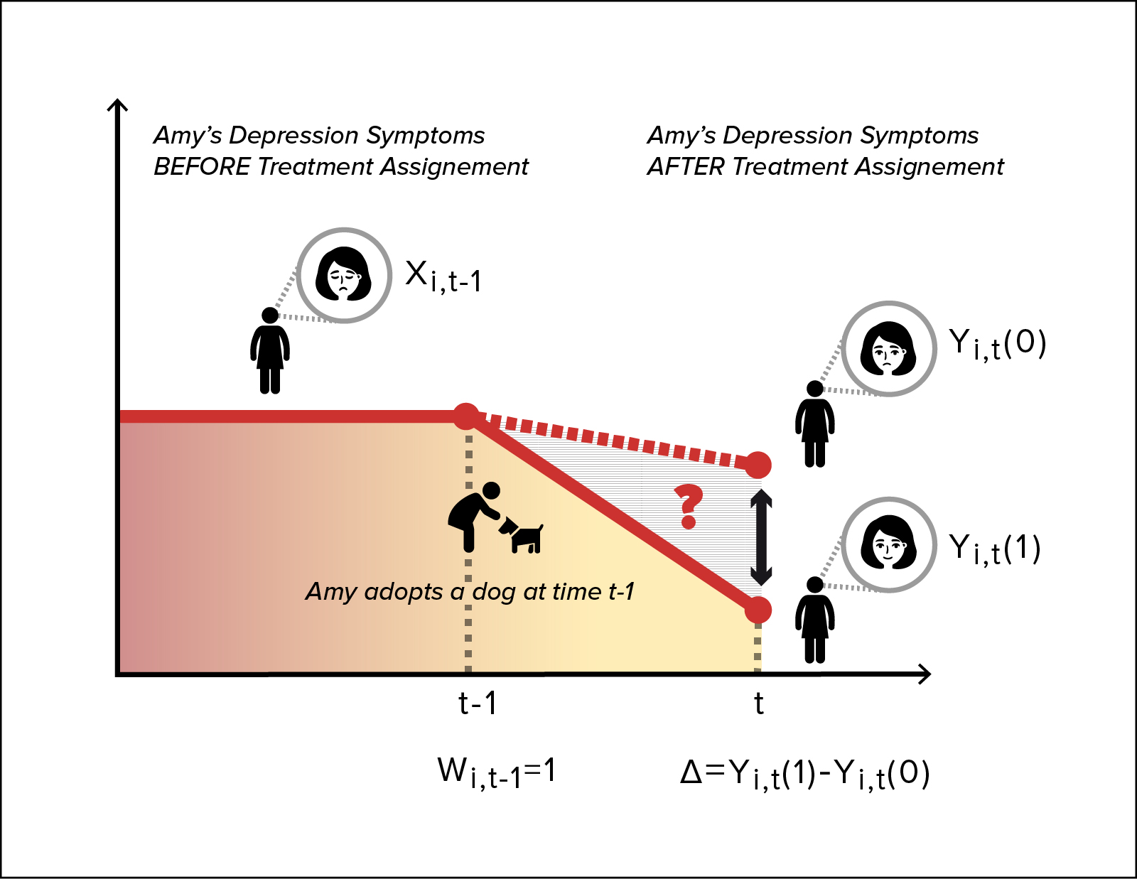
The potential outcomes framework underpins all doubly robust methods. For each individual, define:
- : the outcome that would be observed under treatment ()
- : the outcome that would be observed under control ()
Only one potential outcome is ever observed. The observed outcome links to the potential outcomes through:
The target estimand is the average treatment effect (ATE):
Assumptions for causal inference
Three assumptions must hold for these methods to identify causal effects:
- Consistency: the observed outcome for an individual equals the potential outcome under the treatment they actually received. No hidden versions of treatment.
- Positivity: every individual has a non-zero probability of receiving each treatment level, given their covariates. If some subgroup always gets treated, you can't estimate what would have happened without treatment for that subgroup.
- Conditional exchangeability (no unmeasured confounding): treatment assignment is independent of potential outcomes given the measured covariates . All confounders are captured in .
Inverse probability weighting
Propensity score estimation
The propensity score is the probability of receiving treatment given observed covariates:
It's typically estimated with logistic regression, though machine learning methods (random forests, gradient boosting) are also used. The propensity score serves to balance the covariate distribution between treatment and control groups: within strata of similar propensity scores, treated and untreated individuals should look comparable on observed covariates.
Weighted estimators
The IPW estimator for the ATE is:
Each individual's outcome is weighted by the inverse of their probability of receiving the treatment they actually got. This creates a pseudo-population where treatment assignment is independent of covariates, so a simple weighted comparison of outcomes estimates the ATE.
Limitations of IPW
- Entirely dependent on correct specification of the propensity score model. If that model is wrong, the weights are wrong, and the estimate is biased.
- Extreme weights arise when propensity scores are near 0 or 1, inflating the variance and making estimates unstable. A single observation with gets a weight of 100.
- IPW doesn't model the outcome at all, so it can't leverage information about the outcome-covariate relationship to improve precision.
Outcome regression
Regression adjustment
Outcome regression directly models the expected outcome as a function of treatment and covariates. You fit separate models for each treatment group:
Then for each individual, predict their outcome under both treatment conditions (regardless of which they actually received) and average the differences:
Limitations of outcome regression
- Relies on correct specification of the outcome model. With high-dimensional or nonlinear data, getting this right is hard.
- Doesn't directly balance covariates between groups, so the estimate depends heavily on the model's ability to extrapolate.
- Extrapolation bias is a real concern: if treated individuals have covariate values rarely seen among controls, the outcome model is predicting outside its training data.
Doubly robust estimators
Combining IPW and outcome regression
Doubly robust estimators use both the propensity score and the outcome model in a single estimating equation. The key insight is that the outcome model "augments" the IPW estimator: when the propensity score model is slightly off, the outcome model compensates, and vice versa.
The result is an estimator that's consistent if either model is correctly specified. You still want both to be right (that gives you the best performance), but you only need one.
Semiparametric efficiency
When both models are correctly specified, doubly robust estimators achieve the semiparametric efficiency bound. This is the smallest possible asymptotic variance among all regular estimators for the ATE. In practical terms, this means narrower confidence intervals and more precise estimates than you'd get from IPW or outcome regression alone.
Robustness to model misspecification
The double robustness property is especially valuable in observational studies where the true data-generating process is unknown. You're hedging your bets: even if your propensity score model captures the treatment assignment mechanism but your outcome model is wrong (or the reverse), the estimator still converges to the truth. This is a strict improvement over methods that give you only one shot at correct specification.
Augmented inverse probability weighting
Efficient influence function
The efficient influence function (EIF) is the theoretical building block for constructing doubly robust estimators. It characterizes how much a single observation influences the estimator and determines the asymptotic variance.
For the ATE, the EIF is:
where and are the true outcome models and is the true ATE. Notice the structure: the first two terms are IPW-style terms applied to the residuals (not the raw outcomes), and the last terms are the outcome regression estimate. When either model is correct, the "error" terms vanish in expectation.
AIPW estimator
The augmented inverse probability weighting (AIPW) estimator sets the sample average of the EIF to zero:
Here , are estimated outcome models and is the estimated propensity score.
Think of it this way: start with the outcome regression estimate , then add a bias-correction term that uses IPW on the residuals. If the outcome model is perfect, the residuals are zero and the correction vanishes. If the outcome model is wrong but the propensity score is right, the correction fixes the bias.
Comparison to standard IPW
- AIPW is doubly robust; standard IPW is not. IPW fails entirely if the propensity score model is wrong.
- When the outcome model is well-specified, AIPW is more efficient than IPW because the augmentation term reduces variance.
- The augmentation term also stabilizes the estimator against extreme propensity scores, since it operates on residuals rather than raw outcomes. Large weights matter less when the residuals they multiply are small.
Targeted maximum likelihood estimation
TMLE algorithm
Targeted maximum likelihood estimation (TMLE) is a doubly robust procedure that iteratively updates initial model estimates to specifically target the parameter of interest (here, the ATE).
The steps are:
-
Fit initial models: Estimate the outcome model and the propensity score .
-
Compute clever covariate: For each observation, calculate . This covariate encodes the propensity score information.
-
Targeting step: Fit a regression of on using the initial outcome predictions as an offset (on the appropriate link scale, e.g., logit for binary outcomes). This "tilts" the outcome model toward the ATE.
-
Update predictions: Use the fitted coefficient from step 3 to update the outcome model predictions.
-
Estimate the ATE: Compute the ATE as the average difference in updated predictions: , where the starred quantities are the updated predictions.
Steps 2-4 can be iterated until convergence, though in practice one iteration is often sufficient.

Advantages over AIPW
- TMLE is a substitution estimator: the final ATE estimate is always a function of predicted outcomes, which means it respects the natural bounds of the outcome (e.g., probabilities stay between 0 and 1). AIPW can produce estimates outside the parameter space.
- TMLE is a more general framework, applicable to survival analysis, longitudinal data, and other complex settings.
- The targeting step can improve finite-sample stability, particularly when propensity scores are near the boundaries.
Limitations and considerations
- TMLE is more computationally intensive than AIPW due to the iterative updating.
- Performance depends on the choice of initial estimators and convergence criteria for the targeting step.
- Like all doubly robust methods, TMLE relies on the positivity assumption. Near-violations (propensity scores very close to 0 or 1) can still cause instability, though TMLE tends to handle this better than AIPW in practice.
Doubly robust estimation in practice
Model selection and validation
- Use subject matter knowledge to select covariates for both models. Include variables that are confounders (related to both treatment and outcome). Avoid conditioning on instruments or colliders.
- Data-driven approaches like regularization (LASSO, ridge) can help with variable selection, especially in high-dimensional settings.
- Cross-validation is important for assessing model fit. With doubly robust estimators, cross-fitting (sample splitting) is recommended when using flexible machine learning estimators to avoid overfitting bias.
Diagnostics and sensitivity analysis
- Check overlap: plot the propensity score distributions for treated and control groups. Poor overlap signals positivity violations and unreliable estimates.
- Examine the distribution of IPW weights. If a few observations carry enormous weight, consider trimming or truncating extreme propensity scores.
- Run sensitivity analyses: vary the functional form of the models, swap in different estimators (AIPW vs. TMLE), or use formal sensitivity analysis methods for unmeasured confounding (e.g., E-values).
Extensions and variations
- Doubly robust methods extend to multiple treatments, continuous treatments, and time-varying treatments (longitudinal settings).
- Machine learning can be incorporated into both the propensity score and outcome models to capture complex, nonlinear relationships. This is the basis of doubly robust machine learning (DML) and targeted learning frameworks.
- Adaptations exist for specific study designs such as matched cohorts, clustered data, and survey-weighted samples.
Comparison of doubly robust methods
AIPW vs. TMLE
| Feature | AIPW | TMLE |
|---|---|---|
| Double robustness | Yes | Yes |
| Substitution estimator | No | Yes |
| Respects parameter bounds | Not guaranteed | Yes |
| Computational cost | Lower | Higher |
| Generality | ATE and similar | Broad (survival, longitudinal, etc.) |
Both are asymptotically equivalent when both models are correctly specified, achieving the semiparametric efficiency bound.
Efficiency and robustness tradeoffs
- With both models correct, AIPW and TMLE perform identically in large samples.
- With one model misspecified, both remain consistent, but their finite-sample behavior can differ. TMLE's targeting step often provides better stability when propensity scores are extreme.
- Neither method can save you from misspecifying both models. The "doubly robust" label means two chances, not a guarantee.
Guidelines for method choice
- If your setting is straightforward (binary treatment, cross-sectional data, no extreme propensity scores), AIPW is simpler to implement and often sufficient.
- If you're working with bounded outcomes, complex data structures, or want to pair with machine learning (Super Learner), TMLE is the more flexible choice.
- When in doubt, run both. If AIPW and TMLE give similar answers, that's reassuring. If they diverge meaningfully, investigate why: it often points to model misspecification or positivity problems.