Hypothesis testing overview
Hypothesis testing is a statistical method for making decisions about population parameters using sample data. You set up two competing claims, then use probability to decide which one the data support. In causal inference, this is how you assess whether a treatment effect is real or just noise from random variation.
Null and alternative hypotheses
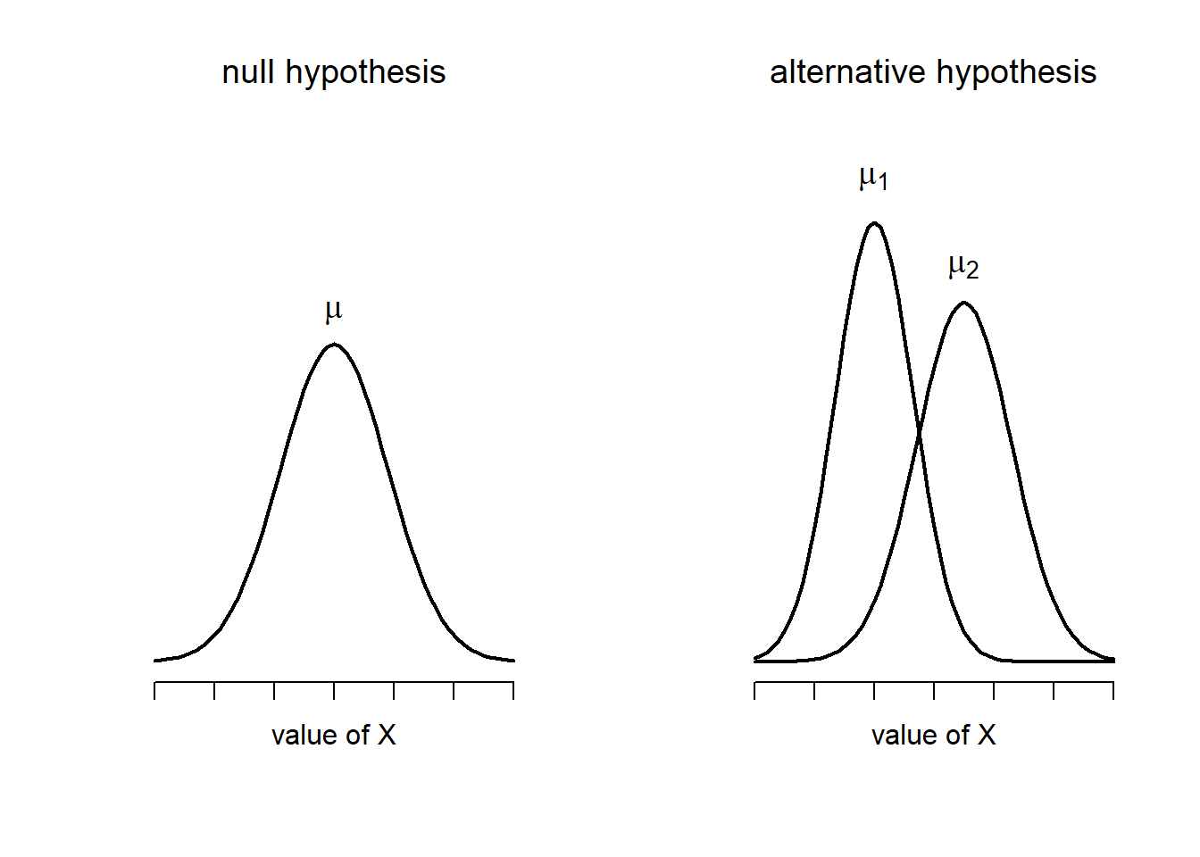
The null hypothesis () represents the default position: no effect, no difference, no relationship. The alternative hypothesis () is the claim you're actually trying to find evidence for.
The logic works like a courtroom. You assume is true (innocent until proven guilty), then ask whether the data are surprising enough to reject that assumption.
- : The mean weight of a population is 150 lbs; : The mean weight is not 150 lbs
- : There is no association between smoking and lung cancer; : There is an association between smoking and lung cancer
Notice that you never "accept" . You either reject it or fail to reject it. Failing to reject just means you didn't find enough evidence against it.
Significance level and p-values
The significance level () is the threshold you set before running the test for how much risk of a false alarm you'll tolerate. Common choices are 0.05 (5%) and 0.01 (1%).
The p-value is the probability of seeing data as extreme as (or more extreme than) what you observed, assuming is true. It is not the probability that is true.
- If , reject . The result is "statistically significant."
- If , fail to reject .
- A smaller p-value means the data are harder to explain under , giving stronger evidence against it.
One-tailed vs two-tailed tests
A two-tailed test checks for any difference in either direction (). It splits across both tails of the distribution.
A one-tailed test checks for a difference in a specific direction ( or ). It puts all of in one tail, making it easier to detect an effect in that direction but blind to effects in the other.
Use a one-tailed test only when you have a strong prior reason to expect the effect goes one way. If you're unsure about direction, go two-tailed.
Type I and Type II errors
These are the two ways a hypothesis test can go wrong:
| is actually true | is actually false | |
|---|---|---|
| Reject | Type I error (false positive) | Correct decision |
| Fail to reject | Correct decision | Type II error (false negative) |
- The probability of a Type I error equals (your significance level).
- The probability of a Type II error is denoted .
- There's a direct trade-off: lowering (being stricter) reduces false positives but increases the chance of missing real effects.
Power of a test
Power is the probability of correctly rejecting when it's actually false. It equals .
A test with low power might fail to detect a real treatment effect, which is a serious problem in causal inference. Four main factors influence power:
- Sample size: Larger samples give more power.
- Effect size: Bigger true effects are easier to detect.
- Significance level: A more lenient (e.g., 0.05 vs 0.01) increases power.
- Variability in the data: Less noise means more power.
Researchers often conduct a power analysis before collecting data to determine the sample size needed to detect a meaningful effect.
Common hypothesis tests
Different tests suit different data types and research questions. The choice depends on whether your data are numerical or categorical, whether you know the population standard deviation, and how many groups you're comparing.
Z-test for population mean
Use the z-test when the population standard deviation () is known and the sample size is large () or the population is normally distributed.
- = sample mean
- = hypothesized population mean
- = population standard deviation
- = sample size
In practice, you rarely know , so the z-test is less common than the t-test. It assumes observations are independent and identically distributed.
T-test for sample mean
Use the t-test when is unknown (which is most of the time). It uses the sample standard deviation instead and accounts for the extra uncertainty with heavier tails in the t-distribution.
The t-test comes in several forms:
- One-sample: Compare a sample mean to a known value.
- Two-sample (independent): Compare means of two separate groups (e.g., treatment vs. control).
- Paired: Compare means from the same subjects measured twice (e.g., before and after treatment).
Assumptions: observations are independent, and the population is approximately normal (though with larger samples, the Central Limit Theorem makes this less critical).
Chi-square test for independence
The chi-square test checks whether two categorical variables are independent. You build a contingency table of observed frequencies and compare them to the frequencies you'd expect if the variables were unrelated.
- = observed frequency in each cell
- = expected frequency in each cell (calculated as row total × column total / grand total)
For example, you might test whether gender and voting preference are independent. A large value means the observed pattern deviates substantially from what independence would predict.
Assumptions: expected frequencies should be at least 5 in each cell, and observations must be independent.
F-test for equality of variances
The F-test compares the variances of two populations to check whether they're equal.
where and are the sample variances. If the populations have equal variances, this ratio should be close to 1.
The F-distribution also underlies ANOVA (analysis of variance), which extends the comparison to three or more group means. Assumptions include normality and independence of observations.
Steps in hypothesis testing
Here's the systematic procedure, from start to finish:
1. Formulating hypotheses
State and clearly based on your research question. They must be mutually exclusive (both can't be true) and exhaustive (one of them must be true). Think carefully about what it would mean to reject in the context of your study.
2. Selecting the appropriate test
Choose a test based on:
- Data type: Numerical → z-test or t-test. Categorical → chi-square.
- What you know: Is known? → z-test. Unknown? → t-test.
- Number of groups: Two groups → t-test. Three or more → ANOVA.
- Direction of hypothesis: One-tailed or two-tailed.
Check whether the test's assumptions (normality, independence, minimum expected counts) are reasonably met.
3. Calculating the test statistic
Plug your sample data into the formula for the test you selected. The test statistic measures how far your sample result is from what predicts, in standardized units.
4. Determining the critical value
Look up the critical value for your chosen and degrees of freedom using a statistical table or software. The critical value marks the boundary of the rejection region.
- For a two-tailed test at , you split the rejection region: 2.5% in each tail.
- For a one-tailed test at , the full 5% goes in one tail.
5. Making the decision
Compare your test statistic to the critical value, or compare your p-value to :
- Test statistic in the rejection region (or ) → reject .
- Test statistic outside the rejection region (or ) → fail to reject .
Always interpret the result in context. "We reject at the 5% level" means something specific about your research question, not just a number comparison.

Interpreting results
Getting a p-value is only half the job. You also need to understand what the result means and what it doesn't mean.
Confidence intervals
A confidence interval gives a range of plausible values for the population parameter. A 95% confidence interval means that if you repeated the study many times, about 95% of the intervals you'd construct would contain the true parameter.
Confidence intervals complement hypothesis tests by showing both the direction and precision of an estimate. A narrow interval means your estimate is precise; a wide one signals more uncertainty. If a 95% CI for a treatment effect doesn't include zero, that's equivalent to rejecting at .
Effect size and practical significance
Statistical significance tells you whether an effect exists. Effect size tells you how big it is. Common measures include:
- Cohen's d: Standardized difference between two means. Values of 0.2, 0.5, and 0.8 are often called small, medium, and large.
- Pearson's r: Correlation coefficient, ranging from -1 to 1.
- Odds ratio: Used in categorical data to compare the odds of an outcome between groups.
Practical significance asks whether the effect matters in the real world. With a large enough sample, you can get a statistically significant p-value for a tiny, meaningless difference. For example, a drug that lowers blood pressure by 0.5 mmHg might be statistically significant with 100,000 participants but clinically irrelevant.
Limitations of hypothesis testing
Hypothesis testing has real weaknesses you should be aware of:
- It does not prove causation on its own. A significant result shows an association, but confounding and reverse causation could still explain it.
- It's sensitive to sample size. Very large samples can make trivially small effects "significant," while small samples may miss important effects.
- Violations of assumptions (non-normality, dependence between observations) can produce misleading results.
- Multiple testing inflates the Type I error rate. If you run 20 tests at , you'd expect about 1 false positive by chance alone. Corrections like Bonferroni adjustment help address this.
Never treat a p-value as the final word. Consider study design, data quality, effect size, and theoretical plausibility alongside your test results.
Applications in causal inference
Hypothesis testing connects directly to the core question of causal inference: did the treatment actually cause the observed outcome, or could the difference be due to chance?
Testing for significant treatment effects
In a randomized controlled trial (RCT), you randomly assign subjects to treatment and control groups, then test whether the difference in outcomes is statistically significant. Randomization is what justifies the causal interpretation: if the groups are comparable at baseline, a significant difference in outcomes can be attributed to the treatment.
For example, testing whether a new drug reduces blood pressure compared to a placebo. If the two-sample t-test yields , you'd reject and conclude the drug has a significant effect (at the 5% level).
Comparing groups in experiments
When experiments involve more than two groups, you need tests that handle multiple comparisons:
- ANOVA tests whether at least one group mean differs from the others.
- Post-hoc tests (like Tukey's HSD) identify which specific pairs of groups differ.
For example, comparing three teaching methods on exam scores. ANOVA might show a significant overall difference, and post-hoc tests would reveal that Method A outperforms Method C but not Method B.
Assessing validity of causal claims
In observational studies and quasi-experiments (where randomization isn't possible), hypothesis testing can evaluate the strength of evidence for a causal relationship. But the results are more ambiguous because you can't rule out confounders the way randomization does.
A significant association between two variables is necessary but not sufficient for a causal claim. You also need to address confounding, selection bias, and reverse causation through study design or statistical adjustment.
Hypothesis testing vs estimation approaches
Hypothesis testing gives you a binary answer: reject or don't reject. Estimation approaches give you richer information:
- Confidence intervals show the range and precision of the estimated effect.
- Bayesian methods incorporate prior knowledge and produce probability distributions over parameter values rather than a single yes/no decision.
In causal inference, the best practice is to use both. Report whether the effect is significant and how large it is with a confidence interval. A treatment effect of 5 points (95% CI: 2 to 8, ) tells you far more than just "."