3.4 Commutation relations and compatible observables

Commutator of Operators

Definition and Properties

The commutator of two operators $\hat{A}$ and $\hat{B}$ is defined as:

$[\hat{A}, \hat{B}] = \hat{A}\hat{B} - \hat{B}\hat{A}$

It measures the extent to which two operators fail to commute. If the commutator is zero, the order you apply the operators doesn't matter. If it's nonzero, the order does matter, and that has direct physical consequences for measurement.

The commutator satisfies several algebraic properties you should know:

• Anticommutativity: $[\hat{A}, \hat{B}] = -[\hat{B}, \hat{A}]$
• Linearity: $[\hat{A}, \hat{B} + \hat{C}] = [\hat{A}, \hat{B}] + [\hat{A}, \hat{C}]$
• Leibniz (product) rule: $[\hat{A}\hat{B}, \hat{C}] = \hat{A}[\hat{B}, \hat{C}] + [\hat{A}, \hat{C}]\hat{B}$
• Self-commutation: $[\hat{A}, \hat{A}] = 0$ always
• Hermiticity property: If $\hat{A}$ and $\hat{B}$ are both Hermitian, then $[\hat{A}, \hat{B}]^\dagger = -[\hat{A}, \hat{B}]$, meaning the commutator is anti-Hermitian

That last point is worth pausing on. Since the commutator of two Hermitian operators is anti-Hermitian, multiplying it by $i$ yields a Hermitian operator. This is exactly what happens with the canonical commutation relation below.

Fundamental Commutation Relations

These are commutation relations you'll use constantly:

• Position-momentum (canonical): $[\hat{x}, \hat{p}] = i\hbar$. This is the most fundamental commutation relation in quantum mechanics and encodes the wave-like nature of quantum particles.
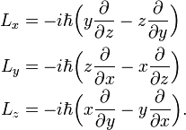
• Angular momentum components: $[\hat{L}_x, \hat{L}_y] = i\hbar \hat{L}_z$ (and cyclic permutations). The components of orbital angular momentum don't commute with each other.
• Spin components: $[\hat{S}_x, \hat{S}_y] = i\hbar \hat{S}_z$ (and cyclic permutations). Spin obeys the same algebra as orbital angular momentum.
• Harmonic oscillator ladder operators: $[\hat{a}, \hat{a}^\dagger] = 1$. This relation is the starting point for the algebraic treatment of the quantum harmonic oscillator.

Physical Significance of Commutation Relations

Quantum Observables and Measurements

Commutation relations tell you something concrete about measurement: whether two observables can be simultaneously known with arbitrary precision.

• If $[\hat{A}, \hat{B}] = 0$, the observables are compatible. You can measure both simultaneously without any fundamental limitation on precision.
• If $[\hat{A}, \hat{B}] \neq 0$, the observables are incompatible. Measuring one disturbs the other, and the uncertainty principle sets a hard lower bound on the product of their uncertainties.

The canonical relation $[\hat{x}, \hat{p}] = i\hbar$ is the reason position and momentum can't both be known exactly. The $i\hbar$ on the right-hand side isn't just a mathematical curiosity; it quantifies the fundamental incompatibility between these two observables.

For angular momentum, the commutation algebra $[\hat{L}_i, \hat{L}_j] = i\hbar \epsilon_{ijk} \hat{L}_k$ determines the entire structure of angular momentum eigenstates, including the allowed quantum numbers $l$ and $m_l$.

Symmetries and Conservation Laws

Commutation relations connect directly to conservation laws through the time evolution of expectation values. If an observable $\hat{A}$ has no explicit time dependence, its time evolution is governed by:

$\frac{d}{dt}\langle \hat{A} \rangle = \frac{i}{\hbar}\langle [\hat{H}, \hat{A}] \rangle$

So if $[\hat{H}, \hat{A}] = 0$, the expectation value of $\hat{A}$ is constant in time, meaning $A$ is a conserved quantity. This is the quantum-mechanical version of Noether's theorem.

Practical consequences:

• Commutation with the Hamiltonian identifies conserved quantities (e.g., $[\hat{H}, \hat{L}_z] = 0$ in a central potential means $m_l$ is conserved)
• Conserved quantities let you build a complete set of commuting observables (CSCO), which fully labels quantum states with simultaneous eigenvalues
• Selection rules in spectroscopy follow from commutation relations between the Hamiltonian and the relevant transition operators

Compatibility of Observables

Criteria for Compatibility

Two observables $\hat{A}$ and $\hat{B}$ are compatible if and only if $[\hat{A}, \hat{B}] = 0$. Here's what that means physically:

1. Compatible observables share a complete set of simultaneous eigenstates. You can find states that are eigenstates of both operators at once.
2. The order of measurement doesn't matter. Measuring $A$ then $B$ gives the same statistical results as measuring $B$ then $A$.
3. After measuring $A$ and obtaining a definite value, a subsequent measurement of $B$ won't disturb the value of $A$.

For incompatible observables ($[\hat{A}, \hat{B}] \neq 0$):

• There is no complete set of simultaneous eigenstates. Some eigenstates of $\hat{A}$ will not be eigenstates of $\hat{B}$.
• The order of measurement matters. Measuring $A$ then $B$ generally gives different results than $B$ then $A$.
• The magnitude of the commutator tells you how incompatible the observables are.

Examples of Compatible and Incompatible Observables

Compatible pairs (commutator equals zero):

• $\hat{L}^2$ and $\hat{L}_z$: You can simultaneously know the total angular momentum and its $z$-component. This is why hydrogen atom states are labeled by both $l$ and $m_l$.
• $\hat{H}$ and $\hat{L}_z$ in a central potential: Energy and the $z$-component of angular momentum are simultaneously well-defined.
• $\hat{L}_z$ and $\hat{S}_z$: The $z$-components of orbital and spin angular momentum commute because they act on different degrees of freedom.

Incompatible pairs (nonzero commutator):

• $\hat{x}$ and $\hat{p}$: The canonical pair. Their commutator $i\hbar$ gives rise to the Heisenberg uncertainty relation.
• $\hat{L}_x$ and $\hat{L}_y$: Different components of angular momentum don't commute. You can't simultaneously know $L_x$ and $L_y$ with arbitrary precision.
• $\hat{S}_x$ and $\hat{S}_y$: Same story for spin components along different axes.

Uncertainty Principle for Incompatible Observables

Mathematical Formulation

The generalized uncertainty principle states that for any two observables $\hat{A}$ and $\hat{B}$:

$\Delta A \, \Delta B \geq \frac{1}{2} \left| \langle [\hat{A}, \hat{B}] \rangle \right|$

where $\Delta A = \sqrt{\langle \hat{A}^2 \rangle - \langle \hat{A} \rangle^2}$ is the standard deviation of $A$ in the given state.

This inequality is a direct mathematical consequence of the noncommutativity of the operators. The commutator on the right-hand side sets the floor.

Key special cases:

• Position-momentum: $[\hat{x}, \hat{p}] = i\hbar$ gives $\Delta x \, \Delta p \geq \frac{\hbar}{2}$. The right-hand side is state-independent here because the commutator is a constant.
• Angular momentum: $[\hat{L}_x, \hat{L}_y] = i\hbar \hat{L}_z$ gives $\Delta L_x \, \Delta L_y \geq \frac{\hbar}{2} |\langle \hat{L}_z \rangle|$. Notice the bound is state-dependent: it depends on $\langle \hat{L}_z \rangle$.
• Energy-time: $\Delta E \, \Delta t \geq \frac{\hbar}{2}$. This one is different because time is not an operator in standard quantum mechanics. The $\Delta t$ here refers to the timescale over which the expectation value of some observable changes appreciably.

Implications and Applications

The uncertainty principle isn't a statement about measurement apparatus being imprecise. It's a fundamental property of quantum states themselves. A state simply cannot have both a sharply defined position and a sharply defined momentum.

Physical consequences include:

• Atomic stability: An electron confined near a nucleus (small $\Delta x$) must have large $\Delta p$, giving it kinetic energy that prevents collapse into the nucleus.
• Natural linewidths: An excited atomic state with a short lifetime (small $\Delta t$) has a spread in energy (large $\Delta E$), which produces a finite linewidth in emission spectra.
• Quantum tunneling: A particle can have enough momentum uncertainty to penetrate a classically forbidden barrier, as seen in alpha decay.
• Zero-point energy: The harmonic oscillator ground state has $E = \frac{1}{2}\hbar\omega$ rather than zero, because confining a particle to the potential minimum would violate the uncertainty principle.