3.2 Magnitude and phase response

Frequency Response Characteristics

Magnitude and Phase Response

When you pass a sinusoidal signal through a linear system, two things happen to it: the amplitude changes and the signal gets shifted in time. Magnitude and phase response capture exactly these two effects across all frequencies.

Magnitude response is the ratio of output amplitude to input amplitude at each frequency. If $|H(j\omega)| = 2$ at some frequency, the system doubles the amplitude of a sinusoid at that frequency. If $|H(j\omega)| = 0.1$, it attenuates it to one-tenth.

Phase response is the angle $\angle H(j\omega)$ at each frequency, measured in degrees or radians. A phase of $-90°$ means the output sinusoid is delayed by a quarter cycle relative to the input. Phase shift generally varies with frequency, which is why you need to examine it across the whole spectrum.

Together, these two quantities fully describe the transfer function evaluated on the $j\omega$ axis:

$H(j\omega) = |H(j\omega)|\, e^{\,j\angle H(j\omega)}$

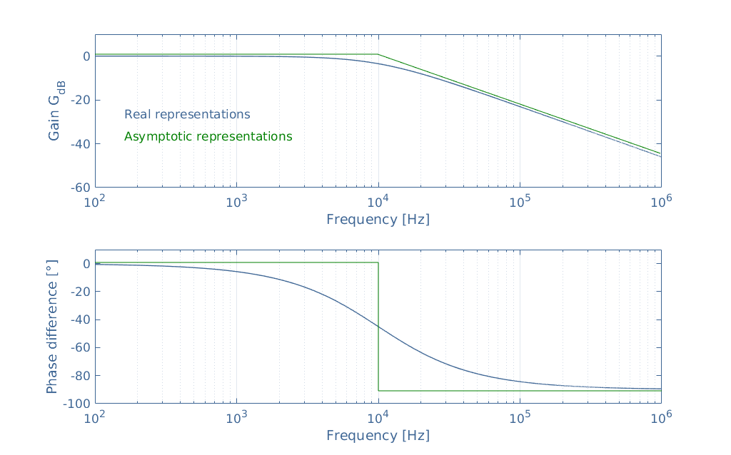
Both are visualized using Bode plots, which display magnitude and phase on separate graphs sharing a common frequency axis.

Decibel and Logarithmic Scales

Magnitude response is almost always expressed in decibels (dB) rather than as a raw ratio. The conversion is:

$|H(j\omega)|_{\text{dB}} = 20 \log_{10} |H(j\omega)|$

A few reference points worth memorizing:

• $|H| = 1 \;\Rightarrow\; 0 \text{ dB}$ (no change in amplitude)
• $|H| = 2 \;\Rightarrow\; \approx 6 \text{ dB}$
• $|H| = 10 \;\Rightarrow\; 20 \text{ dB}$
• $|H| = 0.5 \;\Rightarrow\; \approx -6 \text{ dB}$
• $|H| = \frac{1}{\sqrt{2}} \;\Rightarrow\; -3 \text{ dB}$ (the classic half-power point)

The dB scale compresses a huge dynamic range into manageable numbers. A system whose gain varies from 0.001 to 1000 spans only $-60$ dB to $+60$ dB.

The frequency axis on a Bode plot uses a logarithmic scale (typically in rad/s, sometimes Hz). This lets you see behavior across multiple decades of frequency on a single plot, which is essential because most systems of interest span several decades.

Frequency Domain Parameters

Cutoff Frequency and Bandwidth

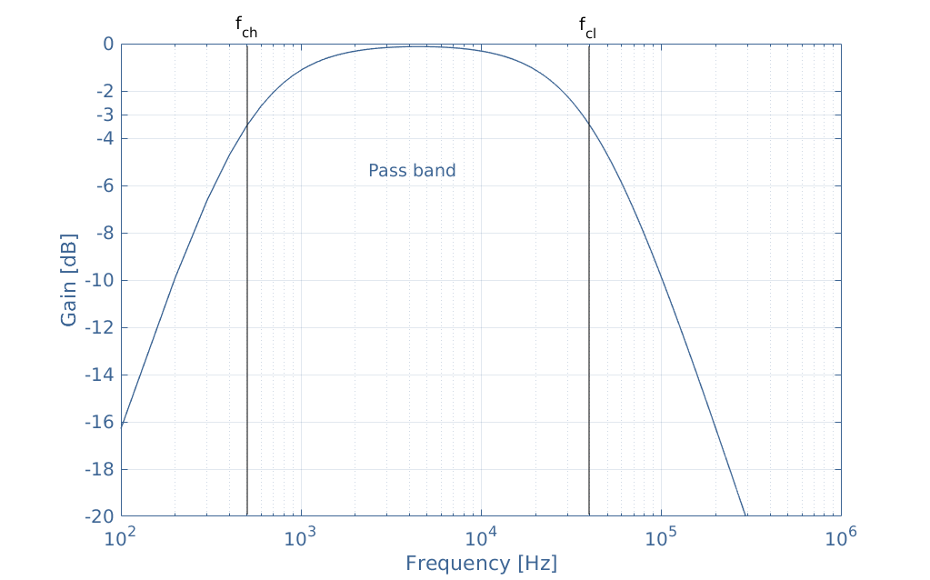
The cutoff frequency ($\omega_c$ or $f_c$) is the frequency at which the magnitude response drops to $-3$ dB relative to its passband value. This corresponds to the half-power point, where $|H(j\omega_c)| = \frac{1}{\sqrt{2}}$ times the passband gain.

How cutoff frequency applies depends on the filter type:

• Low-pass filter: signals below $\omega_c$ pass through with minimal attenuation; signals above $\omega_c$ are increasingly attenuated.
• High-pass filter: signals above $\omega_c$ pass; signals below are attenuated.
• Bandpass filter: has both a lower cutoff $\omega_{c1}$ and an upper cutoff $\omega_{c2}$. Only frequencies between them pass through.

Bandwidth is the range of frequencies a system passes effectively. For a bandpass system:

$BW = \omega_{c2} - \omega_{c1}$

For a low-pass filter, the bandwidth is simply $\omega_c$ (measured from DC). Wider bandwidth generally means the system can handle faster signal transitions and higher data rates.

Resonance and Quality Factor

Resonance occurs when the input frequency matches a system's natural frequency, producing a peak in the magnitude response. In an RLC circuit, for example, the resonant frequency is:

$\omega_0 = \frac{1}{\sqrt{LC}}$

At resonance, reactive impedances cancel, and the response is governed primarily by resistive losses.

The quality factor ($Q$) quantifies how sharp that resonance peak is:

$Q = \frac{\omega_0}{BW}$

• High $Q$ (e.g., $Q = 50$): narrow, pronounced peak. The system responds strongly at $\omega_0$ but rejects nearby frequencies. Think of a highly selective bandpass filter.
• Low $Q$ (e.g., $Q = 0.5$): broad, gentle peak (or no visible peak at all). The system passes a wide range of frequencies without strong selectivity.

The relationship between $Q$ and bandwidth is inverse: doubling $Q$ halves the bandwidth around $\omega_0$.

Stability Margins

Phase Margin and Gain Margin

When analyzing closed-loop systems, you need to know how close the system is to instability. Phase margin and gain margin are the two standard metrics for this, both read directly from the open-loop Bode plot.

Phase margin (PM) is the additional phase lag the system can tolerate before the total loop phase reaches $-180°$. To find it:

1. Locate the gain crossover frequency $\omega_{gc}$, where the open-loop magnitude plot crosses $0$ dB.
2. Read the phase at $\omega_{gc}$. Call it $\phi_{gc}$.
3. Calculate: $PM = 180° + \phi_{gc}$

Since $\phi_{gc}$ is typically negative, a phase of $-135°$ gives $PM = 45°$.

Gain margin (GM) is how much the open-loop gain could increase before the system becomes unstable. To find it:

1. Locate the phase crossover frequency $\omega_{pc}$, where the open-loop phase plot crosses $-180°$.
2. Read the magnitude at $\omega_{pc}$. Call it $|H(j\omega_{pc})|_{\text{dB}}$.
3. Calculate: $GM = 0 - |H(j\omega_{pc})|_{\text{dB}}$

If the gain at $\omega_{pc}$ is $-10$ dB, the gain margin is $+10$ dB.

If either margin is negative or zero, the closed-loop system is unstable or right on the edge of instability.