14.1 Capital budgeting techniques

Capital budgeting techniques are the tools businesses use to evaluate whether an investment project is worth pursuing. They help you compare projects, account for the time value of money, and weigh risk against potential returns.

No single technique gives the full picture. NPV, IRR, Payback Period, and other methods each highlight different aspects of a project's value, so firms typically use several together before committing capital.

Investment Project Evaluation

Net Present Value (NPV) and Internal Rate of Return (IRR)

Net Present Value (NPV) answers a straightforward question: after accounting for the time value of money, does this project create or destroy value?

You calculate NPV by discounting all expected future cash flows back to the present, then subtracting the initial investment:

$NPV = \sum_{t=1}^{n} \frac{CF_t}{(1+r)^t} - \text{Initial Investment}$

where $CF_t$ is the cash flow at time $t$, $r$ is the discount rate, and $n$ is the number of periods.

• A positive NPV means the project is expected to generate more value than it costs, so it's worth considering.
• A negative NPV means the project destroys value at that discount rate.
• The discount rate is typically the firm's weighted average cost of capital (WACC), which represents the minimum return the firm needs to satisfy its investors.

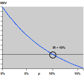
Internal Rate of Return (IRR) is the discount rate that makes a project's NPV exactly zero:

$0 = \sum_{t=1}^{n} \frac{CF_t}{(1+IRR)^t} - \text{Initial Investment}$

Think of IRR as the project's implied rate of return. If the IRR exceeds your required rate of return (usually WACC), the project clears the hurdle. IRR can't be solved algebraically in most cases; you'll use a financial calculator, spreadsheet, or trial and error.

Payback Period and Discounted Payback Period

Payback Period measures how long it takes to recover your initial investment from the project's cash inflows. For projects with equal annual cash flows:

$\text{Payback Period} = \frac{\text{Initial Investment}}{\text{Annual Cash Inflow}}$

It's simple and intuitive, and it tells you something useful about liquidity risk. But it has two major blind spots: it ignores the time value of money, and it completely ignores any cash flows that arrive after the payback date. A project that pays back in 2 years but generates massive returns in years 3 through 10 looks the same as one that stops producing after year 2.

Discounted Payback Period fixes the first problem by discounting each year's cash flow before adding it to the cumulative total. You find the point where cumulative discounted cash flows equal the initial investment. It's more accurate, but it still ignores post-payback cash flows.

Comparison and Interpretation of Methods

These methods can point in different directions, so understanding their strengths matters.

NPV is generally considered the most reliable because it:

• Accounts for the time value of money
• Considers all cash flows over the project's entire life
• Directly measures dollar value created for the firm

IRR gives you a percentage return, which makes it easy to communicate and compare across projects of different sizes. However, it has limitations:

• Projects with non-conventional cash flows (signs that flip more than once) can produce multiple IRRs, making interpretation ambiguous.
• IRR implicitly assumes that interim cash flows are reinvested at the IRR itself, which is often unrealistic. NPV assumes reinvestment at the discount rate, which is usually more conservative and more reasonable.

Payback Period is best used as a quick screening tool or when liquidity is a primary concern. It doesn't measure profitability or long-term value creation.

Capital Budgeting Techniques

Advanced Techniques and Ratios

Profitability Index (PI) expresses value creation as a ratio rather than a dollar amount:

$PI = \frac{\text{Present Value of Future Cash Flows}}{\text{Initial Investment}}$

A PI greater than 1 means the project creates value (its NPV is positive). PI is especially useful under capital rationing, when you have more good projects than available funds, because it ranks projects by value per dollar invested.

Accounting Rate of Return (ARR) uses accounting profit instead of cash flows:

$ARR = \frac{\text{Average Annual Accounting Profit}}{\text{Average Investment}}$

ARR is easy to compute from financial statements, but it ignores the time value of money and relies on accounting figures that can be distorted by depreciation methods and other non-cash items. It's the weakest of the standard techniques for decision-making purposes.

Real Options Analysis recognizes that managers have flexibility after a project begins. You might expand a successful project, delay investment until uncertainty resolves, or abandon a failing one. Traditional NPV treats a project as a fixed commitment; real options analysis values that managerial flexibility using option pricing models (like Black-Scholes or binomial trees). It's more complex and harder to communicate, but it can be critical for projects in highly uncertain environments.

Sensitivity and Scenario Analysis

Capital budgeting outputs are only as good as the assumptions behind them. These techniques help you stress-test those assumptions.

• Sensitivity analysis changes one variable at a time (sales volume, input costs, discount rate) while holding everything else constant. This reveals which variables have the biggest impact on NPV or IRR. If a 5% drop in sales volume swings your NPV from positive to negative, that variable deserves close attention.
• Scenario analysis changes multiple variables simultaneously to model coherent situations: a best case, a worst case, and a most likely case. This gives you a range of outcomes rather than a single point estimate.
• Monte Carlo simulation takes this further by assigning probability distributions to uncertain variables and running thousands of iterations. The output is a full distribution of possible NPVs or IRRs, showing you not just what could happen but how likely each outcome is. It's most useful for complex projects with many interacting uncertainties.

Limitations and Considerations

Every capital budgeting technique rests on assumptions that may not hold:

• NPV and IRR treat future cash flows as if they're known. In practice, they're estimates subject to significant uncertainty.
• Payback Period and ARR ignore the time value of money, which can lead to poor decisions on long-term projects.
• All methods require forecasts about future economic conditions, market demand, competition, and technology, none of which are guaranteed.

Beyond these technical limits:

• Capital rationing (limited funds) may force you to rank and select among projects rather than accepting every positive-NPV opportunity. PI becomes especially valuable here.
• Non-financial factors often matter as much as the numbers: strategic fit, environmental impact, regulatory compliance, and social responsibility can all influence whether a financially attractive project actually gets approved.

Optimal Capital Budgeting Decisions

Integrating Financial Metrics and Strategic Considerations

Good capital budgeting decisions combine quantitative analysis with strategic judgment. A project with the highest NPV isn't automatically the best choice if it doesn't align with the firm's direction.

Strategic factors to weigh alongside financial metrics:

• Market positioning: Does the project strengthen your current market or open a new one?
• Competitive advantage: Does it support cost leadership, differentiation, or innovation?
• Long-term alignment: Does it fit the company's core competencies and growth strategy?

Economic Value Added (EVA) offers another lens on value creation:

$EVA = \text{Net Operating Profit After Taxes} - (\text{Invested Capital} \times WACC)$

A positive EVA means the project earns more than the cost of the capital tied up in it. Unlike NPV, which is a one-time calculation, EVA can be tracked year over year to monitor whether a project continues to create value.

Risk Assessment and Management

Risk assessment goes beyond calculating a single NPV. You need to understand how uncertain your estimates are and what you can do about it.

Risk assessment techniques (covered in more detail above):

• Sensitivity analysis for identifying critical variables
• Scenario analysis for evaluating coherent alternative futures
• Monte Carlo simulation for probabilistic modeling

Risk mitigation strategies:

• Diversification across projects or markets to avoid concentration risk
• Hedging specific exposures like currency fluctuations or commodity prices
• Staged investment (phased commitments) to limit downside if early results disappoint

When projects carry different levels of risk, you should adjust the discount rate accordingly. A riskier project gets a higher discount rate, which raises the bar for acceptance. This risk-adjusted NPV gives a more honest comparison between a safe project and a speculative one.

Non-Financial Factors and Constraints

Financial metrics capture a lot, but not everything. Projects also need to be evaluated on:

• Environmental impact: Carbon footprint, resource use, waste generation, and exposure to future environmental regulations or carbon pricing
• Social responsibility: Effects on communities, employees, and supply chain partners; reputational risks and benefits
• Regulatory and legal compliance: Industry-specific rules, international trade laws, and the likelihood of regulatory changes
• Operational constraints: Whether the firm has the production capacity, supply chain infrastructure, and human capital to execute the project

Time Value of Money in Investments

Fundamental Concepts and Calculations

The time value of money is the foundation beneath every capital budgeting technique. The core idea: a dollar today is worth more than a dollar in the future, because today's dollar can be invested to earn a return, and inflation erodes purchasing power over time.

Two directions of calculation:

Present Value (PV) pulls a future amount back to today:

$PV = \frac{FV}{(1+r)^n}$

Future Value (FV) pushes a current amount forward in time:

$FV = PV \times (1+r)^n$

where $r$ is the interest (or discount) rate and $n$ is the number of periods.

• Compounding moves values forward. Example: $\$1{,}000$ invested at 5% for 3 years grows to $\$1{,}000 \times (1.05)^3 = \$1{,}157.63$.
• Discounting moves values backward. That same $\$1{,}157.63$ received in 3 years is worth $\$1{,}000$ today at a 5% discount rate.

Applications in Investment Decision-Making

Choosing the right discount rate is critical. It should reflect:

• The opportunity cost of capital (what you could earn on the next-best alternative investment)
• The risk level of the specific project (riskier cash flows warrant a higher rate)

Inflation adds another layer. You need to be consistent: discount nominal cash flows (which include inflation) at nominal rates, and real cash flows (inflation-adjusted) at real rates. Mixing them produces incorrect results.

Equivalent Annual Cost (EAC) solves a common comparison problem: how do you choose between projects with different lifespans? EAC converts each project's total NPV of costs into an equivalent annual amount, putting them on the same footing:

$EAC = \frac{NPV}{\dfrac{1-(1+r)^{-n}}{r}}$

where $NPV$ is the net present value of all costs, $r$ is the discount rate, and $n$ is the project's lifespan. The project with the lower EAC is the cheaper option on an annual basis.