6.3 Feedback control systems

Feedback control systems are the backbone of autonomous vehicles, enabling precise control and decision-making in dynamic environments. These systems continuously monitor and adjust vehicle behavior based on real-time sensor data, ensuring safe and efficient operation.

Understanding feedback control principles is crucial for developing robust autonomous vehicle systems. From closed-loop systems to PID controllers and stability analysis, these concepts form the foundation for advanced vehicle control strategies.

Fundamentals of feedback control

• Feedback control systems form the backbone of autonomous vehicle technology, enabling precise control and decision-making in dynamic environments
• These systems continuously monitor and adjust vehicle behavior based on real-time sensor data, ensuring safe and efficient operation
• Understanding feedback control principles is crucial for developing robust and responsive autonomous vehicle systems

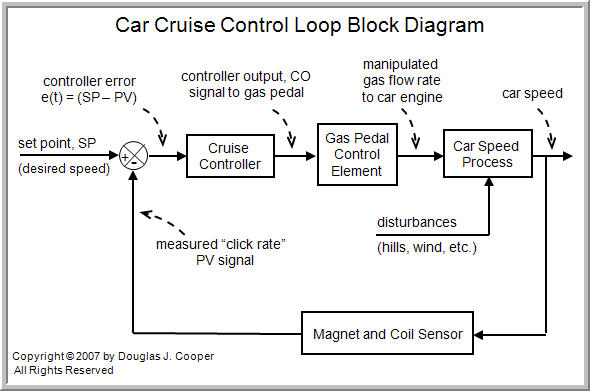
Closed-loop vs open-loop systems

• Closed-loop systems incorporate feedback to adjust output based on measured errors
• Open-loop systems operate without feedback, relying solely on predetermined inputs
• Closed-loop systems offer improved accuracy and disturbance rejection compared to open-loop systems
• Autonomous vehicles primarily utilize closed-loop control for tasks like steering and speed regulation

Components of feedback control systems

• Sensors measure system output and environmental conditions (GPS, cameras, LIDAR)
• Controllers process sensor data and determine appropriate actions (onboard computers)
• Actuators execute control commands to modify system behavior (steering, braking, acceleration)
• Reference inputs define desired system states or trajectories
• Feedback paths transmit measured outputs back to the controller for comparison

Block diagrams and transfer functions

• Block diagrams visually represent system components and their interconnections
• Transfer functions mathematically describe input-output relationships in the frequency domain
• $G(s) = \frac{Y(s)}{U(s)}$ represents the general form of a transfer function
• Block diagram algebra simplifies complex systems into equivalent reduced forms
• Transfer functions enable analysis of system stability, steady-state behavior, and dynamic response

Types of feedback controllers

• Various controller types exist to address different control challenges in autonomous vehicles
• Selection of appropriate controllers depends on system complexity, performance requirements, and environmental conditions
• Advanced control strategies often combine multiple controller types to achieve optimal performance

Proportional-Integral-Derivative (PID) controllers

• Widely used in industry due to simplicity and effectiveness
• Consists of three terms: proportional (P), integral (I), and derivative (D)
• P term provides immediate response to errors
• I term eliminates steady-state errors
• D term improves transient response and stability
• PID control law: $u(t) = K_p e(t) + K_i \int_0^t e(\tau) d\tau + K_d \frac{de(t)}{dt}$

Model predictive control

• Utilizes system model to predict future behavior and optimize control actions
• Solves constrained optimization problem over a finite time horizon
• Handles multivariable systems and explicit constraints effectively
• Particularly useful for autonomous vehicle path planning and obstacle avoidance
• Requires significant computational resources for real-time implementation

Adaptive control systems

• Automatically adjust controller parameters to maintain performance in changing conditions
• Self-tuning controllers estimate system parameters online
• Model reference adaptive control (MRAC) adjusts controller to match desired reference model
• Adaptive control improves robustness to variations in vehicle dynamics and environmental factors

Stability analysis

• Stability analysis ensures autonomous vehicle control systems remain stable under various operating conditions
• Stable systems converge to equilibrium points or desired trajectories when perturbed
• Multiple methods exist for analyzing stability in both time and frequency domains

Routh-Hurwitz criterion

• Determines stability of linear time-invariant systems without solving characteristic equation
• Constructs Routh array from coefficients of characteristic equation
• System is stable if all elements in first column of Routh array have the same sign
• Number of sign changes in first column indicates number of unstable poles
• Provides necessary and sufficient conditions for stability of linear systems

Root locus method

• Graphical technique for analyzing how system poles move as a parameter varies
• Plots loci of closed-loop poles as loop gain changes from 0 to infinity
• Reveals stability margins and dominant pole locations
• Useful for designing feedback controllers and adjusting system gain
• Root locus shape provides insights into system damping and natural frequency

Nyquist stability criterion

• Determines closed-loop stability based on open-loop frequency response
• Plots open-loop transfer function G(s)H(s) in complex plane as s traverses Nyquist contour
• Encirclements of -1 point indicate presence of unstable closed-loop poles
• Provides both absolute and relative stability information
• Particularly useful for systems with time delays or non-minimum phase behavior

Frequency response analysis

• Frequency response analysis examines system behavior under sinusoidal inputs of varying frequencies
• Reveals important system characteristics such as bandwidth, resonance, and stability margins
• Critical for designing robust control systems for autonomous vehicles

Bode plots

• Graphical representation of system magnitude and phase response versus frequency
• Magnitude plot shows system gain in decibels (dB) across frequency range
• Phase plot displays phase shift between input and output signals
• Bode plots facilitate controller design and stability analysis
• Crossover frequency and slope provide insights into system bandwidth and order

Gain and phase margins

• Gain margin measures additional gain system can tolerate before instability
• Phase margin indicates additional phase lag system can handle before instability
• Larger margins generally indicate more robust stability
• Gain margin measured at phase crossover frequency (phase = -180°)
• Phase margin measured at gain crossover frequency (magnitude = 0 dB)

Bandwidth and resonance

• Bandwidth defines frequency range over which system effectively responds to inputs
• Higher bandwidth generally indicates faster system response
• Resonance occurs when system exhibits peak in magnitude response
• Resonant frequency and peak magnitude characterize system damping
• Trade-off exists between bandwidth, stability margins, and noise sensitivity

State-space representation

• State-space models describe system dynamics using first-order differential equations
• Particularly useful for analyzing and controlling multiple-input multiple-output (MIMO) systems
• Enables advanced control techniques such as optimal control and state estimation

State variables and equations

• State variables represent minimum set of system variables to describe its internal condition
• State equations describe how state variables evolve over time
• Output equations relate state variables to system outputs
• General form of continuous-time state-space model: $\dot{x} = Ax + Bu$ $y = Cx + Du$
• A, B, C, and D matrices define system dynamics, input influence, output mapping, and feedthrough

Controllability and observability

• Controllability determines ability to drive system to any desired state using available inputs
• Observability assesses possibility of determining initial state from output measurements
• Controllability matrix: $C = [B \quad AB \quad A^2B \quad ... \quad A^{n-1}B]$
• Observability matrix: $O = [C^T \quad (CA)^T \quad (CA^2)^T \quad ... \quad (CA^{n-1})^T]^T$
• System is controllable if rank(C) = n, observable if rank(O) = n, where n is number of state variables

State feedback design

• Places closed-loop poles at desired locations to achieve required performance
• Feedback gain matrix K computed using pole placement or optimal control techniques
• Closed-loop system with state feedback: $\dot{x} = (A - BK)x$
• Full state feedback requires all state variables to be measured or estimated
• Observer (state estimator) can be designed if not all states are directly measurable

Digital control systems

• Digital control systems use discrete-time signals and computer-based controllers
• Essential for implementing advanced control algorithms in autonomous vehicles
• Offer flexibility, improved noise immunity, and ability to implement complex control laws

Sampling and discretization

• Continuous-time signals converted to discrete-time through sampling process
• Sampling rate must satisfy Nyquist criterion to avoid aliasing
• Zero-order hold (ZOH) commonly used to reconstruct continuous signals from discrete samples
• Discretization methods (Euler, bilinear transform) convert continuous-time models to discrete-time
• Sampling introduces delay and potential instability, requiring careful design considerations

Z-transform and discrete transfer functions

• Z-transform is discrete-time equivalent of Laplace transform
• Maps difference equations to algebraic equations in z-domain
• Discrete transfer function G(z) represents input-output relationship in z-domain
• Stability analysis performed using z-plane (unit circle) instead of s-plane
• Relationship between s-plane and z-plane: $z = e^{sT}$, where T is sampling period

Digital controller design

• Direct digital design develops controller directly in discrete-time domain
• Emulation method converts continuous-time controller to discrete-time equivalent
• Discrete PID controller implementation: $u(k) = K_p e(k) + K_i T \sum_{i=0}^k e(i) + K_d \frac{e(k) - e(k-1)}{T}$
• State-space methods (pole placement, LQR) applicable to discrete-time systems
• Anti-windup techniques prevent integral term saturation in discrete PID controllers

Nonlinear control techniques

• Nonlinear control addresses challenges posed by inherent nonlinearities in vehicle dynamics
• Essential for handling complex behaviors in autonomous vehicles, especially during extreme maneuvers
• Provides improved performance and stability compared to linear control in certain scenarios

Feedback linearization

• Transforms nonlinear system into linear form through nonlinear state feedback
• Input-output linearization focuses on linearizing input-output relationship
• Full-state feedback linearization achieves linear dynamics for entire state space
• Requires accurate system model and full state measurement or estimation
• Enables application of linear control techniques to nonlinear systems

Sliding mode control

• Robust control method that forces system trajectories onto a sliding surface
• Provides insensitivity to matched uncertainties and disturbances
• Control law consists of equivalent control and switching term
• Chattering phenomenon can occur due to imperfect switching
• Boundary layer technique or higher-order sliding modes reduce chattering effects

Backstepping control

• Recursive design procedure for stabilizing strict-feedback and pure-feedback systems
• Breaks down complex nonlinear problem into sequence of simpler design steps
• Constructs Lyapunov function to ensure stability at each step
• Allows for systematic incorporation of nonlinear damping terms
• Particularly useful for underactuated systems and those with non-minimum phase zeros

Robust control methods

• Robust control techniques ensure stability and performance in presence of uncertainties
• Critical for autonomous vehicles operating in diverse and unpredictable environments
• Trade-off exists between robustness and nominal performance

H-infinity control

• Minimizes H-infinity norm of closed-loop transfer function
• Provides robust stability and performance against worst-case disturbances
• Formulated as optimization problem with frequency-dependent weighting functions
• Solutions obtained through solving algebraic Riccati equations or linear matrix inequalities
• Effective for multivariable systems with unstructured uncertainties

Mu-synthesis

• Extends H-infinity control to handle structured uncertainties
• Iteratively solves H-infinity problem and updates uncertainty structure
• Aims to minimize structured singular value (μ) of closed-loop system
• Provides less conservative designs compared to pure H-infinity control
• Computationally intensive, may require model order reduction techniques

Linear quadratic regulator (LQR)

• Optimal control technique minimizing quadratic cost function
• Cost function balances state regulation and control effort
• Solution obtained by solving algebraic Riccati equation
• Provides guaranteed stability margins for continuous-time systems
• LQG (Linear Quadratic Gaussian) combines LQR with Kalman filter for output feedback
• Discrete-time LQR applicable to digital control systems

Control system performance

• Performance metrics quantify how well control system meets design specifications
• Trade-offs exist between different performance criteria (speed vs. overshoot)
• Performance analysis guides controller tuning and system optimization

Steady-state error analysis

• Evaluates system's ability to track constant or time-varying reference inputs
• Static error constants (position, velocity, acceleration) characterize steady-state behavior
• Type of system (0, 1, 2) determines ability to track different input classes with zero error
• Final value theorem used to compute steady-state error for step, ramp, and parabolic inputs
• Integral control action eliminates steady-state error for step inputs in Type 0 systems

Transient response characteristics

• Describe system behavior during transition between steady states
• Key metrics include rise time, settling time, peak time, and percent overshoot
• Second-order system response often used as benchmark for higher-order systems
• Natural frequency and damping ratio influence transient response shape
• Step response analysis reveals important information about system dynamics and stability

Disturbance rejection and noise attenuation

• Measures system's ability to maintain performance in presence of external disturbances
• Sensitivity function S(s) quantifies effect of disturbances on system output
• Complementary sensitivity function T(s) indicates closed-loop response to reference inputs
• Disturbance rejection improved by increasing loop gain at disturbance frequencies
• Noise attenuation achieved by reducing high-frequency gain (low-pass filtering)

Applications in autonomous vehicles

• Feedback control systems play crucial role in various autonomous vehicle subsystems
• Integration of multiple control loops ensures safe, efficient, and comfortable vehicle operation
• Advanced control techniques address challenges posed by complex vehicle dynamics and uncertain environments

Steering control systems

• Maintain vehicle heading and execute desired path following
• Utilize sensors (GPS, IMU, cameras) to determine vehicle position and orientation
• Implement path tracking algorithms (pure pursuit, Stanley method) for trajectory following
• Adaptive steering control compensates for varying road conditions and vehicle speeds
• Steer-by-wire systems enable advanced control strategies and improved responsiveness

Adaptive cruise control

• Maintains desired vehicle speed while adjusting for traffic conditions
• Uses radar or LIDAR to measure distance and relative velocity of leading vehicle
• Implements car-following models to determine appropriate acceleration/deceleration
• Combines longitudinal control with collision avoidance functionality
• Cooperative adaptive cruise control (CACC) incorporates vehicle-to-vehicle communication

Lane keeping assistance

• Detects lane markings using computer vision techniques
• Estimates vehicle position within lane and calculates lateral offset
• Applies corrective steering torque to maintain vehicle within lane boundaries
• Combines with steering control for complete lateral vehicle control
• Advanced systems handle curved roads and absent lane markings

Vehicle stability control

• Enhances vehicle stability during cornering and emergency maneuvers
• Utilizes yaw rate sensors and lateral accelerometers to detect unstable behavior
• Selectively applies individual wheel brakes to correct vehicle motion
• Integrates with traction control and anti-lock braking systems (ABS)
• Advanced systems incorporate active suspension and torque vectoring for improved performance