Linear transformations are like magical machines that turn vectors into other vectors. The kernel and range are two key parts of these machines. They help us understand what goes in and what comes out.
The kernel tells us which vectors become zero, while the range shows all possible outputs. These concepts are super important for figuring out if a transformation is one-to-one or covers everything. They're the building blocks for understanding linear transformations.
Kernel and Range of Linear Transformations
Defining Kernel and Range
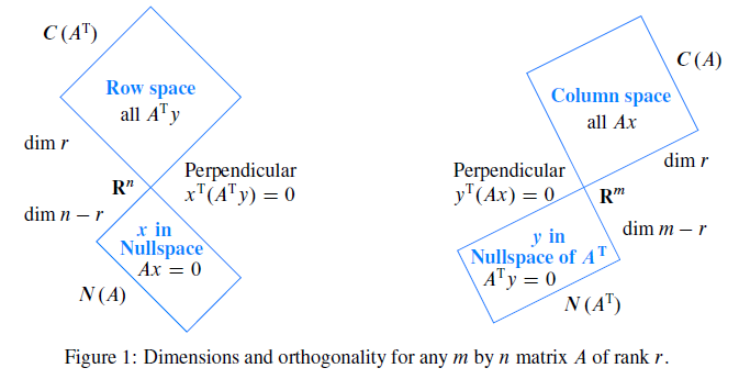
- Kernel (null space) of linear transformation T: V → W encompasses vectors in V mapped to zero vector in W
- Mathematical definition of kernel denoted as ker(T) = {v ∈ V | T(v) = 0}
- Range (image) of linear transformation T: V → W includes all vectors in W that are outputs of T for some input vector in V
- Mathematical definition of range denoted as range(T) = {w ∈ W | ∃v ∈ V, T(v) = w}
- Both kernel and range form subspaces of their respective vector spaces
- Dimension of kernel called nullity of T, dimension of range called rank of T
- Rank-Nullity Theorem states dim(V) = dim(ker(T)) + dim(range(T)) for linear transformation T: V → W
Properties and Relationships
- Kernel provides information about preimage of zero vector in codomain
- Range reveals set of all possible outputs of transformation
- Nullity of injective linear transformation equals zero
- Rank of surjective linear transformation equals dimension of codomain
- Relationship between kernel, range, and injectivity/surjectivity crucial for understanding isomorphisms between vector spaces
- For finite-dimensional vector spaces, injectivity linked to full column rank of matrix representation
- For finite-dimensional vector spaces, surjectivity linked to full row rank of matrix representation
Determining Kernel and Range
Finding the Kernel
- Solve homogeneous equation T(v) = 0 to determine kernel
- For matrix transformations, solving kernel involves homogeneous system Ax = 0 (A represents T)
- Use Gaussian elimination to find basis for kernel
- Express solution as set of vectors
- Verify nullity (dimension of kernel) adheres to Rank-Nullity Theorem

Determining the Range
- Apply transformation to basis of domain
- Express resulting vectors as spanning set
- For matrix transformations, range equals column space of matrix A representing T
- Use Gaussian elimination to determine dimension of range (rank)
- Verify rank adheres to Rank-Nullity Theorem
- Analyze relationship between domain, codomain, and range to understand transformation properties
Examples and Applications
- Linear transformation T: defined by T(x, y, z) = (x + y, y - z)
- Kernel: solve T(x, y, z) = (0, 0) to get ker(T) = {(t, -t, -t) | t ∈ }
- Range: apply T to basis vectors (1, 0, 0), (0, 1, 0), (0, 0, 1) to get range(T) = span{(1, 1), (1, -1)}
- Rotation matrix R =
- Kernel: ker(R) = {(0, 0)} (only zero vector)
- Range: range(R) = (entire codomain)
Kernel and Injectivity
Relationship Between Kernel and Injectivity
- Linear transformation T injective (one-to-one) if and only if kernel contains only zero vector
- Non-injective T implies existence of distinct vectors v1 and v2 in V where T(v1) = T(v2)
- Non-zero vector v1 - v2 in kernel indicates lack of injectivity
- Injectivity determined by analyzing dimension of kernel or rank of transformation matrix
- Nullity of injective linear transformation equals zero

Examples and Applications
- Identity transformation I: V → V always injective (kernel contains only zero vector)
- Projection transformation P: defined by P(x, y, z) = (x, y) not injective
- ker(P) = {(0, 0, t) | t ∈ } (non-zero vectors in kernel)
- Linear transformation T: defined by T(x, y) = (x, y, x+y) injective
- ker(T) = {(0, 0)} (only zero vector in kernel)
Range and Surjectivity
Relationship Between Range and Surjectivity
- Linear transformation T surjective (onto) if and only if range equals codomain
- Non-surjective T implies existence of vector w in W not in range of T
- Surjectivity determined by comparing dimension of range to dimension of codomain
- Rank of surjective linear transformation equals dimension of codomain
Examples and Applications
- Linear transformation T: defined by T(x, y, z) = (x + y, y - z) surjective
- range(T) = (entire codomain)
- Projection transformation P: defined by P(x, y, z) = (x, y) surjective
- range(P) = (entire codomain)
- Linear transformation T: defined by T(x, y) = (x, y, x+y) not surjective
- range(T) = {(a, b, c) ∈ | c = a + b} (proper subspace of )