12.2 Runge-Kutta Methods

Runge-Kutta methods are powerful tools for solving differential equations numerically. They offer a balance between accuracy and computational efficiency, making them essential for tackling complex problems in science and engineering.

These methods use weighted sums of increments to approximate solutions, with higher-order methods providing better accuracy. From the basic fourth-order RK4 to advanced adaptive techniques, Runge-Kutta methods are versatile and widely applicable in various fields.

Runge-Kutta Methods for IVPs

Fundamentals of Runge-Kutta Methods

• Runge-Kutta methods approximate solutions of ordinary differential equations (ODEs) with given initial conditions
• General form involves weighted sum of increments, each increment calculated as product of step size and estimated solution slope
• Derived by matching Taylor series expansion of true solution with numerical approximation up to certain order of accuracy
• Order of method determines local truncation error and relates to number of function evaluations per step
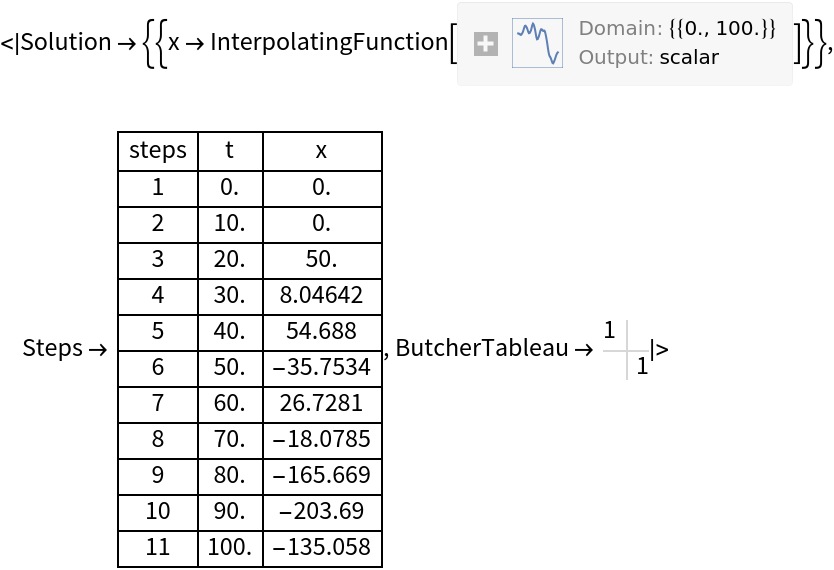
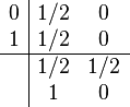
• Butcher tableaus display coefficients and weights used in method (compact representation)
• Explicit methods calculate solution at next time step using only known values
• Implicit methods require solving system of equations at each step
• Apply to systems of ODEs by treating each equation separately and using vector arithmetic

Types and Applications of Runge-Kutta Methods

• Explicit Runge-Kutta methods suitable for non-stiff problems (faster computation)
• Implicit Runge-Kutta methods preferred for stiff problems (better stability properties)
• Symplectic Runge-Kutta methods designed for Hamiltonian systems (preserve important physical properties)
• Embedded Runge-Kutta pairs (Dormand-Prince methods) offer efficient error estimation and adaptive step size control
• Application in various fields (physics, engineering, biology)
  • Modeling planetary motion
  • Simulating chemical reactions
  • Predicting population dynamics

Implementing Fourth-Order Runge-Kutta

RK4 Method Structure

• Fourth-order Runge-Kutta method (RK4) balances accuracy and computational efficiency
• Requires four function evaluations per step to achieve fourth-order accuracy
• Calculates four increments (k1, k2, k3, k4) at different points within each step to estimate solution slope
• Updates solution using weighted average of increments: $y_{n+1} = y_n + \frac{1}{6}(k_1 + 2k_2 + 2k_3 + k_4)$
• Step size selection crucial for balancing accuracy and computational cost
• Adaptive step size techniques automatically adjust step size based on estimated local truncation error
• Applies component-wise to each equation when solving systems of ODEs

RK4 Implementation Considerations

• Choose appropriate initial conditions and step size
• Implement function to evaluate right-hand side of ODE
• Calculate k1, k2, k3, and k4 incrementally within each step
• Update solution using weighted average formula
• Consider error tolerance for adaptive step size methods
• Implement vector operations for systems of ODEs
• Test method on well-known problems with analytical solutions (harmonic oscillator, exponential growth)

Truncation Errors in Runge-Kutta

Local Truncation Error Analysis

• Local truncation error (LTE) introduced in single step of method, assuming all previous values exact
• For s-stage Runge-Kutta method of order p, LTE expressed as $O(h^{p+1})$, where h represents step size
• Estimate LTE using embedded Runge-Kutta pairs
• Richardson extrapolation applied to approximate and reduce local errors
• LTE analysis helps determine appropriate step size for desired accuracy
• Examples of LTE estimation
  • Compare RK4 solution with Taylor series expansion
  • Use embedded Runge-Kutta pair (RK45) to estimate error

Global Truncation Error Analysis

• Global truncation error (GTE) accumulates over all steps from initial point to final solution
• Relationship between local and global truncation errors typically $GTE = O(h^p)$ for method of order p
• Stability analysis studies how errors propagate and potentially amplify over multiple steps
• Richardson extrapolation used to estimate and reduce global errors
• GTE analysis crucial for assessing long-term accuracy of numerical solution
• Examples of GTE analysis
  • Compare numerical solution with known analytical solution over entire interval
  • Use multiple runs with different step sizes to estimate convergence rate

Efficiency vs Accuracy of Runge-Kutta Methods

Efficiency Metrics

• Efficiency measured by number of function evaluations required per step relative to order of accuracy
• Higher-order methods achieve better accuracy for given step size but require more function evaluations
• Concept of "effective order" compares accuracy achieved by different methods for fixed computational cost
• Explicit methods generally more efficient for non-stiff problems
• Implicit methods preferred for stiff problems due to stability properties
• Embedded Runge-Kutta pairs offer efficient error estimation and adaptive step size control
• Examples of efficiency comparisons
  • Compare RK4 with Euler method for solving predator-prey model
  • Analyze computational cost of implicit vs explicit methods for stiff chemical kinetics problem

Selecting Appropriate Runge-Kutta Methods

• Choice depends on specific problem characteristics, desired accuracy, and available computational resources
• Consider stiffness of ODE system when selecting between explicit and implicit methods
• Evaluate trade-off between accuracy and computational cost for different order methods
• Assess importance of preserving specific physical properties (energy conservation, symplecticity)
• Consider adaptive step size methods for problems with varying timescales
• Examples of method selection
  • Choose symplectic method for long-term simulation of planetary orbits
  • Select adaptive Runge-Kutta method for solving chemical reaction system with widely varying reaction rates