9.1 Definition of Riemann Integral

The Riemann integral is a fundamental concept in calculus, defining how we measure the area under a curve. It's all about breaking up a function into tiny pieces, adding them up, and seeing what happens as those pieces get infinitely small.

This idea connects to the broader study of integration by providing a rigorous way to calculate areas and volumes. Understanding the Riemann integral helps us tackle more complex integration problems and lays the groundwork for advanced calculus concepts.

Riemann Integral for Bounded Functions

Definition and Notation

• The Riemann integral defines the integral of a bounded function $f(x)$ on a closed interval $[a, b]$
• $f(x)$ is bounded on $[a, b]$ if there exist real numbers $m$ and $M$ such that $m \leq f(x) \leq M$ for all $x$ in $[a, b]$
• The Riemann integral of $f(x)$ over $[a, b]$ is denoted as $\int_a^b f(x) dx$
• If the limit of Riemann sums exists for $f(x)$ on $[a, b]$, then $f(x)$ is Riemann integrable on $[a, b]$

Riemann Sums and Integrability

• The Riemann integral is defined as the limit of Riemann sums as the norm of the partition approaches zero, if this limit exists
  • The norm (or mesh) of a partition $P$, denoted as $||P||$, is the length of the largest subinterval in the partition
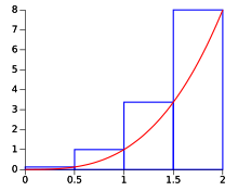
  • The Riemann sum approximates the area under the curve of $f(x)$ over $[a, b]$ by summing the areas of rectangles with heights $f(\xi_i)$ and widths $\Delta x_i$
• A function $f(x)$ is Riemann integrable on $[a, b]$ if and only if for every $\varepsilon > 0$, there exists a $\delta > 0$ such that for any partition $P$ with $||P|| < \delta$ and any choice of sample points, $|S(P, f) - I| < \varepsilon$, where $I$ is the value of the integral

Partitions and Riemann Sums

Partitions and Subintervals

• A partition $P$ of a closed interval $[a, b]$ is a finite set of points $\{x_0, x_1, \ldots, x_n\}$ such that $a = x_0 < x_1 < \ldots < x_n = b$
• The subintervals $[x_{i-1}, x_i]$ for $i = 1, 2, \ldots, n$ are called the subintervals of the partition $P$
  • For example, if $P = \{0, 1, 2, 3\}$ on the interval $[0, 3]$, the subintervals are $[0, 1]$, $[1, 2]$, and $[2, 3]$

Calculating Riemann Sums

• For each subinterval $[x_{i-1}, x_i]$, choose a sample point $\xi_i$ in $[x_{i-1}, x_i]$
• The Riemann sum of $f(x)$ with respect to the partition $P$ and the chosen sample points is defined as $S(P, f) = \sum_{i=1}^n f(\xi_i)\Delta x_i$, where $\Delta x_i = x_i - x_{i-1}$
  • For example, if $f(x) = x^2$ on $[0, 1]$ with partition $P = \{0, 0.5, 1\}$ and sample points $\xi_1 = 0.25$ and $\xi_2 = 0.75$, then $S(P, f) = f(0.25) \cdot 0.5 + f(0.75) \cdot 0.5 = 0.0625 \cdot 0.5 + 0.5625 \cdot 0.5 = 0.3125$

Integrability of Functions

Conditions for Integrability

• Continuous functions on a closed interval $[a, b]$ are always Riemann integrable
  • For example, $f(x) = \sin(x)$ is continuous on any closed interval and thus Riemann integrable
• Monotonic functions on a closed interval $[a, b]$ are always Riemann integrable
  • For example, $f(x) = x^3$ is monotonically increasing on any closed interval and thus Riemann integrable
• Bounded functions with a finite number of discontinuities on a closed interval $[a, b]$ are Riemann integrable
  • For example, $f(x) = \begin{cases} 1, & x \in \mathbb{Q} \\ 0, & x \notin \mathbb{Q} \end{cases}$ is bounded and has infinitely many discontinuities on any interval, so it is not Riemann integrable

Upper and Lower Riemann Integrals

• $f(x)$ is Riemann integrable on $[a, b]$ if and only if the upper and lower Riemann integrals of $f(x)$ over $[a, b]$ are equal
• The upper Riemann integral is the infimum of the upper Riemann sums, while the lower Riemann integral is the supremum of the lower Riemann sums
  • Upper Riemann sum: $U(P, f) = \sum_{i=1}^n \sup_{x \in [x_{i-1}, x_i]} f(x) \Delta x_i$
  • Lower Riemann sum: $L(P, f) = \sum_{i=1}^n \inf_{x \in [x_{i-1}, x_i]} f(x) \Delta x_i$

Computing Riemann Integrals

Using the Definition

• To compute a Riemann integral using the definition, find the limit of Riemann sums as the norm of the partition approaches zero
  • For example, to compute $\int_0^1 x^2 dx$, consider the partition $P_n = \{0, \frac{1}{n}, \frac{2}{n}, \ldots, 1\}$ and the sample points $\xi_i = \frac{i}{n}$. The Riemann sum is $S(P_n, f) = \sum_{i=1}^n (\frac{i}{n})^2 \frac{1}{n} = \frac{1}{n^3} \sum_{i=1}^n i^2$. As $n \to \infty$, this sum approaches $\frac{1}{3}$, which is the value of the integral

Properties of Riemann Integrals

• Linearity: For constants $a$ and $b$, $\int_a^b [af(x) + bg(x)] dx = a\int_a^b f(x) dx + b\int_a^b g(x) dx$
• Additivity: If $c$ is in $[a, b]$, then $\int_a^b f(x) dx = \int_a^c f(x) dx + \int_c^b f(x) dx$
• Monotonicity: If $f(x) \leq g(x)$ for all $x$ in $[a, b]$, then $\int_a^b f(x) dx \leq \int_a^b g(x) dx$

Fundamental Theorem of Calculus

• The Fundamental Theorem of Calculus relates the Riemann integral to the antiderivative of a function, providing a powerful tool for computing integrals
  • If $F(x)$ is an antiderivative of $f(x)$ on $[a, b]$, then $\int_a^b f(x) dx = F(b) - F(a)$
  • For example, since $F(x) = \frac{1}{3}x^3$ is an antiderivative of $f(x) = x^2$, we have $\int_0^1 x^2 dx = F(1) - F(0) = \frac{1}{3} - 0 = \frac{1}{3}$