Seismic reflection and refraction methods are the primary tools geophysicists use to image Earth's subsurface. Both techniques generate seismic waves and record how those waves interact with underground layers, but they exploit different physical phenomena and serve different purposes. Reflection methods capture waves that bounce off subsurface interfaces, producing detailed structural images. Refraction methods capture waves that travel along interfaces, revealing large-scale velocity structure. Understanding how each works, when to use it, and what can go wrong is essential for designing surveys and interpreting results.
Seismic Reflection vs Refraction
Principles and Methods
Seismic reflection measures the two-way travel time of waves that bounce off subsurface interfaces such as sedimentary boundaries and faults. The physical basis is acoustic impedance contrast. Acoustic impedance () is the product of seismic velocity and density:
Whenever a wave crosses an interface where changes significantly, part of its energy reflects back to the surface. The stronger the contrast, the stronger the reflection.
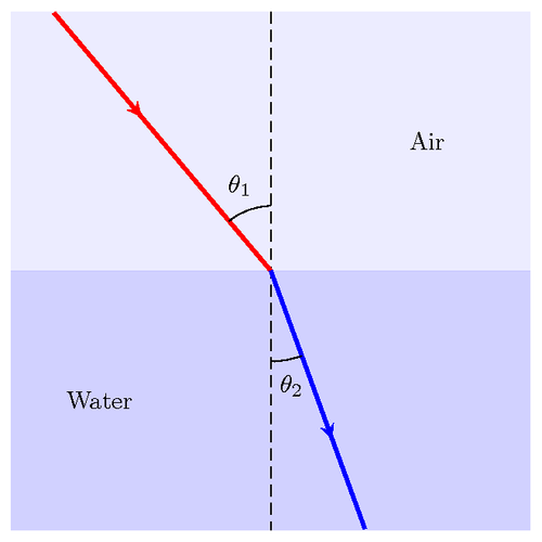
Seismic refraction measures the travel times of waves that are critically refracted along subsurface interfaces. The physical basis is Snell's law, which relates the angles of incidence and refraction at a boundary:
Critical refraction occurs when the refracted ray travels exactly along the interface (). This happens at the critical angle , where . The refracted wave then propagates at the velocity of the faster, deeper layer and radiates energy back to the surface as it goes.
A key requirement for refraction to work: velocity must increase with depth. If a low-velocity layer sits beneath a high-velocity layer, the refracted arrivals from deeper interfaces can be hidden, creating a "hidden layer" problem.
Applications and Survey Design
Reflection and refraction surveys differ in their targets, resolution, and logistics:
| Feature | Reflection | Refraction |
|---|---|---|
| Best for | Detailed imaging of complex structures (basins, reservoirs, faults) | Large-scale velocity structure and crustal layering |
| Receiver spacing | Dense (meters to tens of meters) | Can be wider (hundreds of meters to kilometers) |
| Frequency content | Higher frequencies for better resolution | Lower frequencies that propagate over longer distances |
| Offset range | Moderate (target-dependent) | Long offsets needed to record critically refracted arrivals |
| Processing focus | Deconvolution, stacking, migration | Travel time picking, intercept-time analysis, tomographic inversion |
The choice between methods depends on target depth, the resolution you need, and available budget. Many projects use both: refraction for a velocity framework and reflection for structural detail.
Seismic Survey Design
Survey Planning and Parameter Selection
Designing a seismic survey starts with defining the geologic target. The target's depth, size, and structural complexity drive every parameter choice.
Source selection depends on the environment:
- Land: Explosives (strong, impulsive signal) or vibroseis trucks (controllable, repeatable sweep signal)
- Marine: Air guns towed behind a vessel
Receiver selection also depends on the environment:
- Land: Geophones, which measure ground velocity
- Marine: Hydrophones, which measure pressure changes in water
Key parameter trade-offs:
- Deeper targets require longer source-receiver offsets and lower source frequencies, since high frequencies attenuate more rapidly with distance.
- Higher resolution demands denser spatial sampling (closer receiver spacing) and higher frequencies.
- Fold coverage (the number of traces that share a common midpoint) controls the signal-to-noise ratio after stacking. Higher fold means better noise suppression but more field effort.
Recording parameters like sampling rate, record length, and anti-alias filters should be set to capture the full bandwidth of useful signal without aliasing or truncating reflections from the deepest target.
Survey Logistics and Quality Control
Land surveys face practical constraints that shape the design:
- Rugged terrain may require helicopter-portable equipment or specialized vibroseis vehicles. Survey geometries might shift from regular grids to crooked-line 2D or sparse 3D layouts.
- Environmental regulations can restrict source types (no explosives near wetlands, for example) or limit access during sensitive wildlife seasons.
Marine surveys tow long hydrophone streamers (sometimes 8+ km) behind a vessel, with air gun arrays firing at regular intervals:
- Streamer length and the number of parallel streamers determine subsurface coverage and crossline resolution.
- GPS and acoustic positioning systems track source and receiver locations precisely. Even small positioning errors degrade image quality.
Quality control during acquisition is critical. Field crews monitor source output (consistent signatures), receiver responses (no dead or noisy channels), and ambient noise levels in real time. Data gaps from equipment failures or access problems are much cheaper to fill during acquisition than to work around in processing.
Seismic Data Interpretation

Reflection Data Processing and Imaging
Raw seismic reflection data is noisy and geometrically distorted. Processing transforms it into an interpretable subsurface image. Here's the standard workflow:
- Trace editing — Remove dead, noisy, or corrupted traces that would degrade the final image.
- Amplitude recovery — Compensate for energy loss due to geometric spreading (amplitude decreases with distance) and absorption (the earth converts seismic energy to heat).
- Deconvolution — Compress the source wavelet to sharpen temporal resolution. This removes reverberations and the imprint of the source signature.
- Velocity analysis — Estimate how seismic velocity varies with depth by examining how reflection travel times change with offset. This step is iterative and directly affects image quality.
- Normal moveout (NMO) correction — Reflections from a flat layer arrive later at far offsets than near offsets, forming a hyperbolic curve. NMO correction flattens these hyperbolas so that all traces for a given reflector align at the same time.
- Stacking — Sum all NMO-corrected traces that share a common midpoint (CMP). This boosts the signal (reflections add constructively) and suppresses random noise.
- Migration — Reposition reflectors to their true subsurface locations. Without migration, dipping reflectors appear shifted, and diffraction patterns from faults or pinch-outs remain unresolved. Migration also collapses the Fresnel zone, improving horizontal resolution.
For geologically complex areas (salt bodies, thrust belts), advanced techniques like pre-stack depth migration and full-waveform inversion can produce more accurate images by handling strong lateral velocity variations that simpler methods cannot.
Refraction Data Processing and Velocity Modeling
Refraction processing focuses on extracting velocity and layer-thickness information from first-arrival travel times.
- Pick first arrivals on each trace. These are the earliest arriving energy, typically refracted waves at longer offsets and direct waves at short offsets.
- Plot travel time vs. offset curves. Each straight-line segment on this plot corresponds to a different subsurface layer. The slope of each segment equals , where is the velocity of that layer. The intercept time (where the line extrapolates back to zero offset) relates to the depth and velocity of overlying layers.
- Invert for layer model. Simple cases (flat, horizontal layers) can be solved with intercept-time formulas. More complex structures require tomographic inversion, which iteratively adjusts a velocity model until predicted travel times match observed ones. Two common approaches:
- Ray tracing — Simulates individual ray paths through the model
- Wavefront methods — Solve the eikonal equation to compute travel times across a gridded model
The resulting velocity model is most useful when integrated with other data. Well logs provide ground-truth velocities and lithologies at specific points. Gravity and magnetic data add constraints on density and composition. Seismic attributes extracted from reflection data (amplitude, phase, frequency variations) can further characterize reservoir properties like porosity, lithology, and fluid content.
Seismic Method Limitations
Resolution and Accuracy Constraints
Vertical resolution is governed by the dominant wavelength () of the seismic signal:
where is velocity and is dominant frequency. The commonly cited vertical resolution limit is approximately . For example, at m/s and Hz, m, so vertical resolution is roughly 15 m. Layers thinner than this may still produce a reflection, but you can't resolve their top and bottom as separate interfaces.
Horizontal resolution before migration is limited by the Fresnel zone, the area on a reflector that contributes constructively to a single reflection event. The Fresnel zone radius grows with depth and wavelength. Migration processing collapses the Fresnel zone, sharpening horizontal resolution to roughly half the dominant wavelength under ideal conditions.
Velocity model accuracy depends on the quality of travel time picks, the assumptions built into inversion algorithms (e.g., isotropy, layer geometry), and how well the survey geometry samples the subsurface. Seismic anisotropy, caused by aligned fractures, fine layering, or mineral fabric, makes velocity direction-dependent. If anisotropy isn't accounted for, depth conversions and structural interpretations can contain significant errors.
Geologic Complexity and Interpretation Challenges
Certain geologic settings push seismic methods to their limits:
- Salt bodies have much higher velocities than surrounding sediments and often have irregular shapes. They distort the wavefield passing through them, creating shadow zones and imaging artifacts beneath the salt.
- Volcanic intrusions scatter seismic energy and introduce sharp velocity anomalies, making it difficult to image structures below them.
- Steeply dipping layers may not reflect energy back to the surface receivers (limited illumination), leaving gaps in the image.
Seismic data alone has limited sensitivity to fluid type and pore pressure. Amplitude variation with offset (AVO) analysis can provide some fluid and lithology discrimination by examining how reflection strength changes with offset, but it requires careful calibration. Well logs and core samples remain essential for tying seismic responses to actual rock and fluid properties.
Non-uniqueness is a fundamental challenge: multiple geologic models can produce the same seismic response. A bright reflection could be a gas sand, a coal seam, or a cemented layer. Interpreters constrain their models using regional geologic knowledge, well ties, and complementary geophysical datasets.
Finally, cost and environmental impact can limit where seismic surveys are feasible. Surveys may be restricted near populated areas, in protected habitats, or during sensitive ecological periods. Mitigation measures like low-energy sources, seasonal timing restrictions, and marine mammal observers are increasingly standard practice.