Vector spaces form the foundation of linear algebra, combining vector addition and scalar multiplication. These operations follow specific rules, ensuring consistent behavior across various mathematical structures.
From Euclidean spaces to function spaces, vector spaces appear in many forms. Understanding their axioms and examples is crucial for grasping more advanced concepts in linear algebra and its applications.
Axioms of Vector Spaces
Vector Addition and Scalar Multiplication
Top images from around the web for Vector Addition and Scalar Multiplication File:Vector addition.png - Wikimedia Commons View original
Is this image relevant?
Vectors · Algebra and Trigonometry View original
Is this image relevant?
Vector (mathematics and physics) - Wikipedia View original
Is this image relevant?
File:Vector addition.png - Wikimedia Commons View original
Is this image relevant?
Vectors · Algebra and Trigonometry View original
Is this image relevant?
1 of 3
Vector space V over field F combines two operations
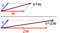
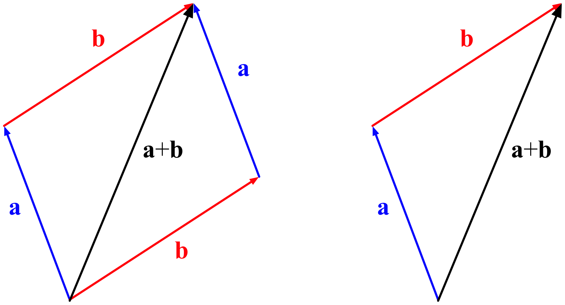
Vector addition (binary operation on V)
Scalar multiplication (operation between F and V elements)
Vector addition exhibits key properties
Commutative u + v = v + u \mathbf{u} + \mathbf{v} = \mathbf{v} + \mathbf{u} u + v = v + u
Associative ( u + v ) + w = u + ( v + w ) (\mathbf{u} + \mathbf{v}) + \mathbf{w} = \mathbf{u} + (\mathbf{v} + \mathbf{w}) ( u + v ) + w = u + ( v + w )
Identity element (zero vector) 0 + v = v \mathbf{0} + \mathbf{v} = \mathbf{v} 0 + v = v
Inverse elements v + ( − v ) = 0 \mathbf{v} + (-\mathbf{v}) = \mathbf{0} v + ( − v ) = 0
Scalar multiplication satisfies distributivity and compatibility
Distributive over vector addition a ( u + v ) = a u + a v a(\mathbf{u} + \mathbf{v}) = a\mathbf{u} + a\mathbf{v} a ( u + v ) = a u + a v
Distributive over scalar addition ( a + b ) v = a v + b v (a + b)\mathbf{v} = a\mathbf{v} + b\mathbf{v} ( a + b ) v = a v + b v
Compatible with field multiplication ( a b ) v = a ( b v ) (ab)\mathbf{v} = a(b\mathbf{v}) ( ab ) v = a ( b v )
Uniqueness and Closure Properties
Zero vector uniqueness ensures single additive identity
Additive inverse uniqueness guarantees v + ( − v ) = 0 \mathbf{v} + (-\mathbf{v}) = \mathbf{0} v + ( − v ) = 0 for each vector
Multiplicative identity of field (typically 1) acts as scalar multiplication identity
1 v = v 1\mathbf{v} = \mathbf{v} 1 v = v for all vectors v
Closure property maintains vector space integrity
Vector addition result always within V
Scalar multiplication result always within V
Examples of Vector Spaces
Finite-Dimensional Spaces
Euclidean spaces Rⁿ (n ≥ 1) over real numbers
Componentwise addition ( x 1 , . . . , x n ) + ( y 1 , . . . , y n ) = ( x 1 + y 1 , . . . , x n + y n ) (x_1, ..., x_n) + (y_1, ..., y_n) = (x_1 + y_1, ..., x_n + y_n) ( x 1 , ... , x n ) + ( y 1 , ... , y n ) = ( x 1 + y 1 , ... , x n + y n )
Scalar multiplication a ( x 1 , . . . , x n ) = ( a x 1 , . . . , a x n ) a(x_1, ..., x_n) = (ax_1, ..., ax_n) a ( x 1 , ... , x n ) = ( a x 1 , ... , a x n )
Polynomial spaces P_n(F) over field F
Degree ≤ n polynomials
Addition ( a 0 + a 1 x + . . . + a n x n ) + ( b 0 + b 1 x + . . . + b n x n ) = ( ( a 0 + b 0 ) + ( a 1 + b 1 ) x + . . . + ( a n + b n ) x n ) (a_0 + a_1x + ... + a_nx^n) + (b_0 + b_1x + ... + b_nx^n) = ((a_0 + b_0) + (a_1 + b_1)x + ... + (a_n + b_n)x^n) ( a 0 + a 1 x + ... + a n x n ) + ( b 0 + b 1 x + ... + b n x n ) = (( a 0 + b 0 ) + ( a 1 + b 1 ) x + ... + ( a n + b n ) x n )
Scalar multiplication c ( a 0 + a 1 x + . . . + a n x n ) = ( c a 0 + c a 1 x + . . . + c a n x n ) c(a_0 + a_1x + ... + a_nx^n) = (ca_0 + ca_1x + ... + ca_nx^n) c ( a 0 + a 1 x + ... + a n x n ) = ( c a 0 + c a 1 x + ... + c a n x n )
Matrix spaces M_m,n(F) over field F
m × n matrices
Addition [ a i j ] + [ b i j ] = [ a i j + b i j ] [a_{ij}] + [b_{ij}] = [a_{ij} + b_{ij}] [ a ij ] + [ b ij ] = [ a ij + b ij ]
Scalar multiplication c [ a i j ] = [ c a i j ] c[a_{ij}] = [ca_{ij}] c [ a ij ] = [ c a ij ]
Infinite-Dimensional Spaces
Continuous function space C[a,b] on interval [a,b]
Pointwise addition ( f + g ) ( x ) = f ( x ) + g ( x ) (f + g)(x) = f(x) + g(x) ( f + g ) ( x ) = f ( x ) + g ( x )
Scalar multiplication ( c f ) ( x ) = c f ( x ) (cf)(x) = cf(x) ( c f ) ( x ) = c f ( x )
Sequence space over field F
Infinite-dimensional vectors (a₁, a₂, a₃, ...)
Componentwise operations
Solution space of homogeneous linear differential equations
Linear combinations of fundamental solutions
Advanced function spaces
L²[a,b] (square-integrable functions)
C∞(R) (infinitely differentiable functions)
Verifying Vector Spaces
Axiom Verification Process
Systematically check all vector space axioms for given set and operations
Verify closure property for vector addition and scalar multiplication
Ensure operations result in elements within the set
Confirm vector addition properties
Commutativity u + v = v + u \mathbf{u} + \mathbf{v} = \mathbf{v} + \mathbf{u} u + v = v + u
Associativity ( u + v ) + w = u + ( v + w ) (\mathbf{u} + \mathbf{v}) + \mathbf{w} = \mathbf{u} + (\mathbf{v} + \mathbf{w}) ( u + v ) + w = u + ( v + w )
Zero vector existence 0 + v = v \mathbf{0} + \mathbf{v} = \mathbf{v} 0 + v = v
Additive inverse existence v + ( − v ) = 0 \mathbf{v} + (-\mathbf{v}) = \mathbf{0} v + ( − v ) = 0
Check scalar multiplication properties
Distributivity over vector addition a ( u + v ) = a u + a v a(\mathbf{u} + \mathbf{v}) = a\mathbf{u} + a\mathbf{v} a ( u + v ) = a u + a v
Distributivity over scalar addition ( a + b ) v = a v + b v (a + b)\mathbf{v} = a\mathbf{v} + b\mathbf{v} ( a + b ) v = a v + b v
Compatibility with field multiplication ( a b ) v = a ( b v ) (ab)\mathbf{v} = a(b\mathbf{v}) ( ab ) v = a ( b v )
Multiplicative identity 1 v = v 1\mathbf{v} = \mathbf{v} 1 v = v
Special Considerations and Challenges
Identify potential counterexamples violating axioms
Non-closure (operation results outside the set)
Lack of commutativity or associativity
Missing or non-unique zero vector or inverses
Prove uniqueness of zero vector and inverse elements
Demonstrate 0 + v = v \mathbf{0} + \mathbf{v} = \mathbf{v} 0 + v = v holds only for one element
Show v + ( − v ) = 0 \mathbf{v} + (-\mathbf{v}) = \mathbf{0} v + ( − v ) = 0 has unique solution for each v
Analyze abstract or non-standard vector spaces carefully
Examine operation definitions closely
Consider implications of unusual scalar fields (finite fields, complex numbers)
Verify scalar multiplication behaves correctly with field operations
Check compatibility with addition and multiplication in the scalar field