1.3 Floating Point Arithmetic and Error Analysis

Floating-point arithmetic is crucial for representing real numbers in computers. It's not perfect though – rounding errors can creep in and mess up calculations. Understanding these limitations helps us avoid nasty surprises in our matrix computations.

Error analysis is all about figuring out how these tiny errors can snowball into bigger problems. We'll look at different types of errors, how they spread through calculations, and clever tricks to keep them in check. This stuff is super important for getting reliable results from our matrix algorithms.

Floating-Point Representation of Numbers

IEEE 754 Standard and Floating-Point Format

Top images from around the web for IEEE 754 Standard and Floating-Point Format

• 

  IEEE 754 - Wikipedia View original

  Is this image relevant?

• 

  Double-precision floating-point format - Wikipedia View original

  Is this image relevant?

• 

  Real number approximations in finite space with IEEE 754 – jeffq, published View original

  Is this image relevant?

• 

  IEEE 754 - Wikipedia View original

  Is this image relevant?

• 

  Double-precision floating-point format - Wikipedia View original

  Is this image relevant?

1 of 3

Top images from around the web for IEEE 754 Standard and Floating-Point Format

• 

  IEEE 754 - Wikipedia View original

  Is this image relevant?

• 

  Double-precision floating-point format - Wikipedia View original

  Is this image relevant?

• 

  Real number approximations in finite space with IEEE 754 – jeffq, published View original

  Is this image relevant?

• 

  IEEE 754 - Wikipedia View original

  Is this image relevant?

• 

  Double-precision floating-point format - Wikipedia View original

  Is this image relevant?

1 of 3

• Floating-point representation approximates real numbers in binary format using sign bit, exponent, and mantissa (significand)
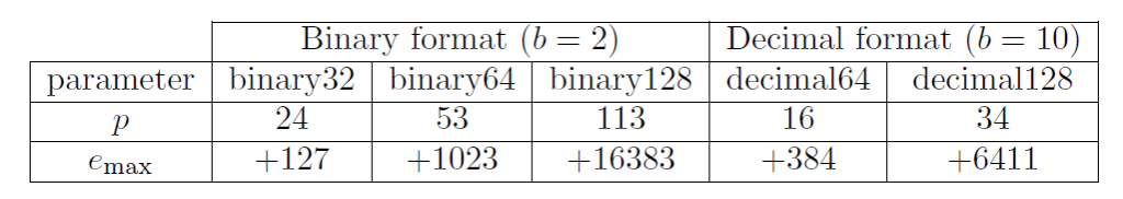
• IEEE 754 standard defines format and rules for floating-point arithmetic
  • Single precision (32-bit) representation
  • Double precision (64-bit) representation
• Normalized floating-point numbers have implicit leading 1 in mantissa to save space
• Special values in floating-point arithmetic
  • Infinity (positive and negative)
  • Not a Number (NaN) for exceptional cases (undefined operations)
• Machine epsilon (εmachine) defines smallest representable difference between 1 and next larger floating-point number
  • Crucial for understanding precision limits in computations

Rounding and Subnormal Numbers

• Rounding modes in floating-point arithmetic
  • Round-to-nearest (default mode)
  • Round-toward-zero
  • Round-toward-positive-infinity
  • Round-toward-negative-infinity
• Subnormal numbers (denormalized numbers) extend range of representable numbers close to zero
  • Allow for gradual underflow
  • Improve precision for very small values
• Examples of rounding effects:
  • $0.1_{10} = 0.00011001100110011..._2$ (recurring in binary)
  • Rounding to nearest in single precision: $0.100000001490116119384765625$

Sources of Errors in Computations

Roundoff and Truncation Errors

• Roundoff errors occur due to finite precision of floating-point representation and arithmetic operations
  • Example: $1/3 \approx 0.333333333333333$ (in double precision)
• Truncation errors arise from approximating infinite processes with finite ones
  • Series expansions (Taylor series)
  • Numerical integration (trapezoidal rule, Simpson's rule)
• Cancellation errors result from subtracting nearly equal numbers, leading to loss of significant digits
  • Example: $(1 - \cos x) / x^2$ for small x

Input and Algorithmic Errors

• Input errors or data uncertainty propagate through calculations and affect final result
  • Measurement errors in experimental data
  • Rounding errors in input values
• Algorithmic errors stem from choice of numerical method or algorithm used to solve a problem
  • Different algorithms for same problem may have varying error characteristics
• Condition number of a problem quantifies its sensitivity to perturbations in input data
  • Well-conditioned problems: small changes in input cause small changes in output
  • Ill-conditioned problems: small changes in input cause large changes in output
• Backward error analysis assesses quality of computed solution
  • Determines size of perturbations to input data that would yield computed result exactly
  • Helps distinguish between problem sensitivity and algorithm stability

Roundoff Error Propagation in Matrices

Error Bounds and Condition Numbers

• Error bounds for basic matrix operations derived using perturbation theory and matrix norms
  • Addition: $\|A + B\| \leq \|A\| + \|B\|$
  • Multiplication: $\|AB\| \leq \|A\| \|B\|$
• Relative error crucial for assessing accuracy of matrix computations
  • Especially important for matrices with widely varying magnitudes of entries
• Condition numbers for matrix operations provide upper bounds on error magnification
  • Matrix inversion: $\kappa(A) = \|A\| \|A^{-1}\|$
  • Solving linear systems: $\kappa(A) = \|A\| \|A^{-1}\|$
• Backward error analysis for matrix computations relates computed solution to exact solution of nearby problem
  • Helps distinguish between problem sensitivity and algorithm stability

Numerical Stability and Error Reduction Techniques

• Scaling techniques improve conditioning of matrix problems and reduce error propagation
  • Row and column scaling to balance matrix entries
• Effects of pivoting strategies in Gaussian elimination on numerical stability
  • Partial pivoting reduces growth factor and improves stability
  • Complete pivoting provides best theoretical bounds but is computationally expensive
• Iterative refinement techniques improve accuracy of computed solutions
  • Compute residual: $r = b - Ax$
  • Solve for correction: $A\delta x = r$
  • Update solution: $x = x + \delta x$
• Example: Solving ill-conditioned system $Ax = b$ with and without iterative refinement

Minimizing and Controlling Numerical Errors

Precision and Algorithm Selection

• Use higher precision arithmetic for intermediate calculations to reduce roundoff errors
  • Example: Using double precision for accumulating single precision results
• Implement numerically stable algorithms that minimize error accumulation and propagation
  • Modified Gram-Schmidt for QR factorization
  • Householder transformations for least squares problems
• Apply preconditioning techniques to improve conditioning of matrix problems before solving
  • Jacobi preconditioning for sparse matrices
  • Incomplete LU factorization for iterative solvers

Advanced Error Control Techniques

• Utilize error estimators and adaptive algorithms to control errors in iterative methods
  • Residual-based error estimators for linear solvers
  • Adaptive step size control in ODE solvers
• Employ mixed precision techniques
  • Use lower precision for bulk computations
  • Use higher precision for critical operations (dot products, accumulations)
• Implement compensated summation algorithms to reduce errors in accumulating floating-point numbers
  • Kahan summation algorithm: $s = s + (y + c)$, where c is a running compensation term
• Develop robust stopping criteria for iterative methods based on both relative residual and error estimates
  • Combine residual-based and solution-based criteria
  • Use multiple convergence checks to ensure reliability